
Geometric Distribution
Loading the math board and drawing, please wait…
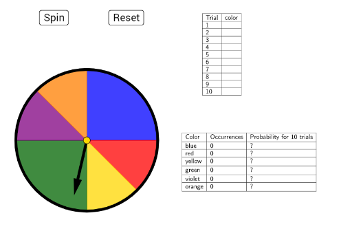
This example demonstrates the probability distribution of a geometric distribution. Key mathematical concepts include the probability calculation of a geometric distribution. Using GeoGebra commands such as CountIf, Circle, Rotate, etc., the probability distribution can be dynamically displayed. Suitable for high school math education or students researching geometric distributions.
GeoGebra Commands & Parameters
CountIf(x ≟ "orange", B2:B11) → E7CountIf(x ≟ "violet", B2:B11) → E6CountIf(x ≟ "green", B2:B11) → E5CountIf(x ≟ "yellow", B2:B11) → E4CountIf(x ≟ "red", B2:B11) → E3CountIf(x ≟ "blue", B2:B11) → E2Circle(A, B) → cRotate(S0, ((-a))°, A) → CVector(A, C) → uLine(B, A) → bOrthogonalLine(A, b) → eIntersect(c, e) → D, ECircleSector(A, E, B) → fIntersect(c, b) → F, GMidpoint(G, E) → HLine(A, H) → gIntersect(c, g) → I, JCircleSector(A, J, E) → hCircleSector(A, G, J) → kCircleSector(A, D, G) → pCircleSector(A, I, D) → qCircleSector(A, B, I) → rIsInRegion(C, f) → iIsInRegion(C, h) → jSum(Sequence[(IsInRegion[C, Element[liste2, k]] * k), k, 1, 6]) → mElement(liste1, m) → texte1TableText({{A1, B1}, {A2, B2}, {A3, B3}, {A4, B4}, {A5, B5}, {A6, B6}, {A7, B7}, {A8, B8}, {A9, B9}, {A10, B10}, {A11, B11}}, "|_") → text1TableText({{D1, E1, F1}, {D2, E2, F2}, {D3, E3, F3}, {D4, E4, F4}, {D5, E5, F5}, {D6, E6, F6}, {D7, E7, F7}}, "|_") → text2
AI Drawing Prompt Reference
Draw a geometric distribution probability distribution. First, calculate the number of data points in each color region based on the given data, and use commands like circles and rotations to dynamically display the geometric distribution probability. Then, construct multiple sectors through a series of circle, rotation, and intersection operations to represent different probability values. Finally, determine the final graphic display by judging the position of points.
The prompt above was compiled from the original drawing commands and is for reference only.