
Geometric Construction of Cylinder–Cone Intersections
Loading the math board and drawing, please wait…
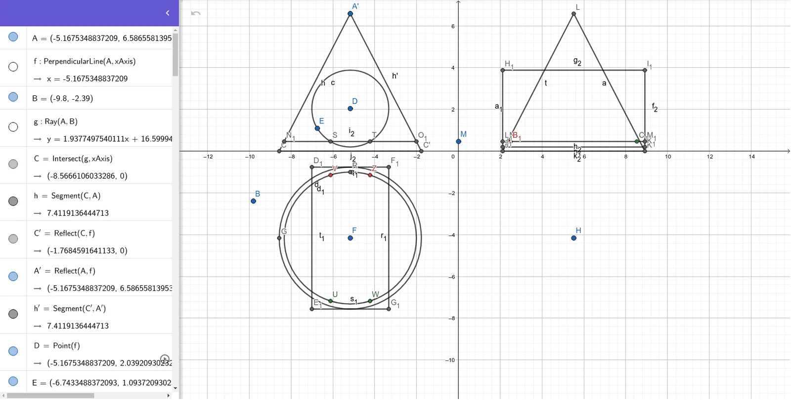
This example demonstrates how the intersection curve of a cylinder and a cone can be reconstructed and visualized while dragging a control (parameter) point. It provides an intuitive way to observe how the spatial intersection changes with configuration. Key concepts include solid geometry of cylinders and cones, intersections between lines/segments in 3D construction workflows, circle-based auxiliary constructions, and tangent constraints. The construction relies on GeoGebra commands listed in the summary: Line and Ray to define supporting directions, Intersect and Segment to compute intersection points, Circle and Tangent to enforce tangency conditions, OrthogonalLine to create perpendicular helpers, and Mirror to use symmetry for building corresponding parts. Using Points and multiple labeled objects (including mirrored/primed counterparts) the model assembles the full intersection geometry. Suitable for high-school to early university learners studying 3D geometry, geometric construction, and visualization for math modeling.
GeoGebra Commands & Parameters
OrthogonalLine(A, xAxis) → fRay(A, B) → gIntersect(g, xAxis) → CSegment(C, A) → hMirror(C, f) → C'Mirror(A, f) → A'Segment(C', A') → h'Point(f) → DCircle(D, E) → cLine(C, f) → iPoint(f) → FLine(F, xAxis) → jIntersect(j, i) → GCircle(F, G) → dTangent(f, c) → k, lTangent(j, d) → m, nPoint(j) → HLine(H, yAxis) → pIntersect(p, n) → ICircle(H, I) → eTangent(p, e) → q, rIntersect(q, xAxis) → JIntersect(r, xAxis) → KLine(A, xAxis) → sIntersect(s, p) → LSegment(J, L) → tSegment(L, K) → aTangent(xAxis, c) → b, f_1Line(M, xAxis) → g_1Intersect(g_1, t) → NLine(N, p) → h_1Intersect(h_1, j) → OCircle(H, O) → c_1Tangent(j, c_1) → i_1, j_1Intersect(i_1, j) → PIntersect(j, i_1) → QIntersect(i_1, f) → RCircle(F, R) → d_1Intersect(c, g_1) → S, TLine(S, f) → k_1Intersect(d_1, k_1) → U, VLine(T, l) → l_1Intersect(d_1, l_1) → W, ZLine(V, j) → m_1Intersect(m_1, p) → A_1Circle(H, A_1) → e_1Tangent(p, e_1) → n_1, p_1Intersect(g_1, n_1) → B_1Intersect(g_1, p_1) → C_1Intersect(m, k) → D_1Intersect(k, n) → E_1Intersect(l, m) → F_1Intersect(n, l) → G_1Segment(D_1, F_1) → q_1Segment(F_1, G_1) → r_1Segment(G_1, E_1) → s_1Segment(E_1, D_1) → t_1Intersect(b, q) → H_1Intersect(b, r) → I_1Intersect(f_1, q) → J_1Intersect(f_1, r) → K_1Segment(H_1, J_1) → a_1Segment(J_1, K_1) → b_1Segment(K_1, I_1) → f_2Segment(I_1, H_1) → g_2Intersect(g_1, a_1) → L_1Intersect(g_1, f_2) → M_1Segment(L_1, M_1) → h_2Intersect(g_1, h) → N_1Intersect(g_1, h') → O_1Segment(N_1, O_1) → i_2Segment(C, C') → j_2Segment(J, K) → k_2
AI Drawing Prompt Reference
Draw a geometric construction in one coordinate system to visualize the intersection geometry between a cylinder and a cone. Use two reference axes, and allow a control parameter point to move so the configuration updates. First, determine several key intersection points on the axes and build auxiliary segments to set endpoints. Create circles centered at selected points, then construct tangents between those circles and the relevant lines to obtain constrained tangency points. Use perpendicular helper lines and mirror symmetry to replicate the corresponding parts on the opposite side. Continue by intersecting several auxiliary lines with each other and with the axes to generate additional circle centers and tangency points. Combine the resulting circles, tangents, and intersection points to form the full reconstructed intersection outline.
The prompt above was compiled from the original drawing commands and is for reference only.