
Finding Perimeter
Loading the math board and drawing, please wait…
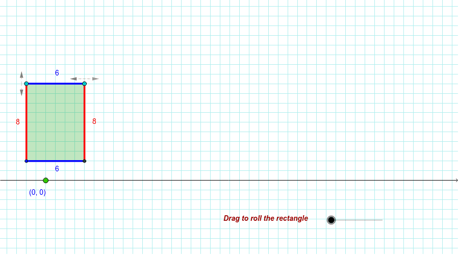
This example demonstrates how to calculate and visualize the perimeter of polygons using GeoGebra. Core mathematical concepts include perimeter calculation, vector operations, and geometric transformations. Key construction elements involve commands and objects like UnitOrthogonalVector, Point, Ray, Segment, Length, Intersect, Rotate, Polygon. Suitable for high school mathematics education, helping students understand and apply methods for calculating polygon perimeters.
GeoGebra Commands & Parameters
UnitOrthogonalVector(xAxis) → vPoint(xAxis) → EIf(i > 0, i, 0) → αIf(i ≤ 0, i, 0) → trRay(L, K) → nPoint(n) → BUnitVector(Segment[B, O]) → uTranslate(B, Vector[(((tr + 1) * u) * Distance[B, O])]) → B'Ray(L, J) → lPoint(l) → ATranslate(A, Vector[(((tr + 1) * u) * Distance[B, O])]) → A'OrthogonalLine(A, l) → bPoint(b) → CTranslate(C, Vector[(((tr + 1) * u) * Distance[B, O])]) → C'Segment(A, C) → cOrthogonalLine(C, c) → dLength(Vector[A, C]) → hSegment(A, B) → aOrthogonalLine(B, a) → eIntersect(d, e) → DTranslate(D, Vector[(((tr + 1) * u) * Distance[B, O])]) → D'Angle(E, O, D') → βIf(α < β, 1, Div[α - β, 1.5708] + 2) → mIf(m ≟ 1, α, α - β - ((m - 2) * 3.141592653589793 / 2)) → AngRLength(Vector[A, B]) → tMax(h, t) → longSequence((Element[list1, k], 0), k, 1, 5) → list2If(m ≟ 1, D', If[Distance[Element[list2, m - 1], Element[list2, m]] ≟ h, Element[list2, m] + (v * t), Element[list2, m] + (v * h)]) → D_1If(m ≟ 1, C', If[Distance[Element[list2, m - 1], Element[list2, m]] ≟ h, Element[list2, m - 1] + (v * t), Element[list2, m - 1] + (v * h)]) → C_1If(m ≟ 1, B', Element[list2, m]) → B_1If(m ≟ 1, A', Element[list2, m - 1]) → A_1Element(list2, m) → centRotate(C_1, (-AngR), cent) → IRotate(D_1, (-AngR), cent) → HRotate(B_1, (-AngR), cent) → GRotate(A_1, (-AngR), cent) → FPolygon(F, G, H, I) → poly3', f_1, g_1, h_1, i_1Line(A, B) → a11Polygon(A, B, D, C) → poly1, a_1, b_1, d_1, c_1Polygon(A', B', D', C') → poly1', a', b', d', c'Append(A', list2) → list3Polygon(A_1, B_1, D_1, C_1) → poly3, a_2, b_2, d_2, c_2Sequence(Segment[Element[list2, k], Element[list2, k + 1]], k, 1, 4) → list4Element(list4, 1) → side1Element(list4, 2) → side2Element(list4, 3) → side3If(f_1 ≟ long, 1, 0) → colorfElement(list4, 4) → side4If(h_1 ≟ long, 1, 0) → colorhIf(g_1 ≟ long, 1, 0) → colorgIf(i_1 ≟ long, 1, 0) → coloriPoint(A, Vector[UnitVector[l]]) → MPoint((x(C), y(C) + 0.5), Vector[UnitVector[c]]) → NIf(side1 ≟ long, 1, 0) → co1If(side2 ≟ long, 1, 0) → co2If(side3 ≟ long, 1, 0) → co3If(side4 ≟ long, 1, 0) → co4Vector((x(A) - 0.5, y(A)), (x(M) - 0.5, y(A) + 1.3)) → fVector((x(A) - 0.5, y(A)), (x(M) - 0.5, y(A) - 1.3)) → zVector((x(C) - 0.5, y(C) + 0.5), (x(N) + 0.5, y(N))) → gVector((x(C) + 0.5, y(C) + 0.5), (x(N) - 2.5, y(N))) → w
AI Drawing Prompt Reference
Visualize the perimeter calculation of a polygon using vector operations and geometric transformations. Start with a base line, construct polygon vertices with orthogonal vectors and rays, then adjust vertex positions through rotations and translations to form a closed polygon. Highlight the sides and key points of the polygon in different colors, and label the perimeter length to intuitively demonstrate the calculation process.
The prompt above was compiled from the original drawing commands and is for reference only.