
F.4 Trigonometric Function (Sine) Dynamic Demo
Loading the math board and drawing, please wait…
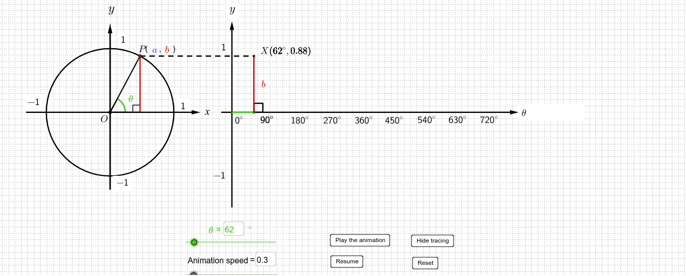
① This example dynamically illustrates the geometric definition of the sine function using a unit circle, showing how the angle maps to a point on the sine curve and how the graph is generated. ② Core mathematical concepts include the sine function, unit circle, angle and radian measure, periodicity, and the relationship between geometric constructions and function graphs. ③ Construction highlights: uses GeoGebra commands such as Segment, Circle, Intersect, Rotate, OrthogonalLine, Point, Ray, Angle, Textfield, Midpoint, Vector, If, and Polygon, with objects like a slider (Play_1) for animation and multiple text fields for dynamic labels. ④ Suitable for senior secondary students (e.g., DSE F.4 or equivalent) learning trigonometry, useful for classroom demonstrations, interactive exploration, and understanding the sine function's geometric origin and graphical representation.
GeoGebra Commands & Parameters
Segment(O, B_1) → h_1Circle(O, 3.141592653589793) → cIntersect(c, h_1) → D_1,Rotate(D_1, x(W), O) → A_2Intersect(xAxis, yAxis) → OriginSegment(Origin, O) → hIntersect(c, h) → D,OrthogonalLine(D, xAxis) → c_1Rotate(D, x(W), O) → AOrthogonalLine(A, xAxis) → gIntersect(g, xAxis) → BSegment(B, O) → kSegment(O, A) → bIntersect(b, k) → ESegment(A_2, O) → b_1Intersect(b_1, c_1) → FOrthogonalLine(Origin, xAxis) → dOrthogonalLine(Origin, d) → fPoint(xAxis) → GRay(Origin, G) → mAngle(D, O, A) → βTextfield(Θ) → inputBox1Segment(O, D) → aOrthogonalLine(A, a) → eSegment(A, B) → jSegment(A, X) → lSegment(W, Origin) → nSegment(X, W) → qSegment(W, Y) → sSegment(W, Z) → tAngle(A, B, O) → γSegment(F, D) → d_1Segment(F, A) → e_1Midpoint(q) → HMidpoint(s) → IMidpoint(t) → SSegment(B, O) → pPoint(yAxis) → PPoint(yAxis) → QVector(P, Q) → uPoint(u) → RPoint(xAxis) → TTextfield(speed) → inputBox2Angle(T, W, X) → δAngle(T, W, Y) → εVector(U, V) → zVector(A_1, B_1) → u_1Vector(A_1, B_1) → v_1Vector(C_1, T) → vVector(V, U) → z_1Segment(A_2, Y) → I_1Angle(D_1, O, A_2) → β_1OrthogonalLine(A_2, xAxis) → g_1Intersect(g_1, xAxis) → B_2Segment(A_2, B_2) → a_1Angle(A_2, B_2, O) → γ_1If(f_1 ≟ 1, true, false) → FAIf(f_1 ≟ 0, true, false) → FBPolygon(E_1, F_1, G_1, H_1) → poly1, e_2, f_2, g_2, h_2
AI Drawing Prompt Reference
Draw a unit circle centered at the origin with radius approximately π. From the center, draw a horizontal ray as the initial side. Place a point on the circle and rotate it by a dynamic angle, showing the angle in radians. Drop a perpendicular from the circle point to the horizontal axis, marking the foot. Connect the center to the circle point to form a radius. Outside the circle, set up coordinate axes and map the y-coordinate of the circle point to the horizontal axis to generate the corresponding point on the sine curve. Add a slider to control the angle and display dynamic text for the angle and sine value. Connect relevant points with segments to form a right triangle, labeling the angle and side relationships.
The prompt above was compiled from the original drawing commands and is for reference only.