
Exponential & Logarithm Graphs
Loading the math board and drawing, please wait…
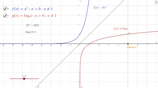
This example demonstrates the graphs of exponential and logarithmic functions. It involves key mathematical concepts such as exponential and logarithmic functions and their properties. Using GeoGebra commands like Point, OrthogonalLine, and Intersect, dynamic constructions of these functions are possible. Suitable for high school mathematics education and learning.
GeoGebra Commands & Parameters
Point(xAxis) → AOrthogonalLine(A, xAxis) → iIntersect(g, i, (3, 0.6826061944859853)) → BPoint(yAxis) → COrthogonalLine(C, yAxis) → jIntersect(f, j, (0.6826061944842778, 2.999999999991756)) → DIf(a > 1, "a>0", If[a < 1, "0<a<1", "ไม่นิยาม"]) → tPoint(xAxis) → ELine(E, yAxis) → kIntersect(f, k, (5, 3125)) → FIntersect(g, k, (5, 1)) → G
AI Drawing Prompt Reference
Draw a coordinate system to display the graphs of exponential and logarithmic functions. Start by plotting the x-axis and y-axis. Take a point on the x-axis and draw a line perpendicular to it; let this line intersect the exponential function graph at a point. Similarly, take a point on the y-axis, draw a line perpendicular to it, and let this line intersect the logarithmic function graph at another point. Based on the value of parameter a, label the properties of the exponential and logarithmic functions. Finally, draw two lines from the origin that intersect the exponential and logarithmic function graphs, and mark the intersection points.
The prompt above was compiled from the original drawing commands and is for reference only.