
Exploring the Relationship Between y = a*cos(bx) + c and y = cos(x)
Loading the math board and drawing, please wait…
This example demonstrates how adjusting parameters a, b, and c transforms the graph of y = a*cos(bx) + c from y = cos(x). Key math concepts include trigonometric function graph transformations, amplitude伸缩, period changes, and vertical shifts. GeoGebra commands/objects like f, g, h, p, q, r, s, t, f_1, g_1, h_1, a, p_1 are used to plot and dynamically adjust the function graphs. Suitable for high school students learning trigonometric function transformations and introductory calculus/analytic geometry.
GeoGebra Commands & Parameters
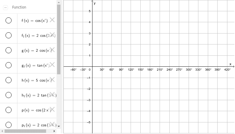
f(x) = cos(x°)g(x) = (2 * cos(x°))h(x) = (5 * cos(x°))p(x) = cos(((2 * x))°)q(x) = cos(((3 * x))°)r(x) = (2 * cos(((3 * x))°))s(x) = cos(x°) + 2t(x) = cos(x°) - 3f_1(x) = (2 * cos(((3 * x))°)) + 1g_1(x) = tan(x°)h_1(x) = (2 * tan(((3 * x))°)) + 1y = 1p_1(x) = (2 * cos(((3 * x))°)) + 1
AI Drawing Prompt Reference
Draw two cosine function graphs, one is the standard cosine function, and the other is a cosine function with amplitude doubled and period halved. Then draw a cosine function with amplitude five times larger. Next, draw cosine functions with periods halved and tripled. Then draw a cosine function with amplitude doubled and period tripled. After that, draw the standard cosine function shifted up by 2 units, and finally draw the standard cosine function shifted down by 3 units, as well as the cosine function with amplitude doubled and period tripled shifted up by 1 unit.
The prompt above was compiled from the original drawing commands and is for reference only.