
Exploring Sine and Cosine of an Angle
Loading the math board and drawing, please wait…
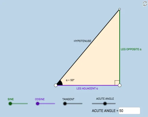
This example demonstrates the dynamic behavior and geometric interpretation of sine and cosine values within a right triangle. It involves core mathematical concepts such as side length relationships in right triangles, definitions of trigonometric functions, and dynamic geometric visualization. The construction utilizes GeoGebra commands like Segment, OrthogonalLine, Rotate, Angle, Ray, Circle, Intersect, Polygon, and Textfield to build the figure and enable interactive exploration. Suitable for high school mathematics education to intuitively understand the connection between trigonometric functions and the sides/angles of right triangles.
GeoGebra Commands & Parameters
Segment(A, B) → fOrthogonalLine(B, f) → gRotate(B, (a * π / 180), A) → B'Angle(B, A, B') → αRay(A, B') → hCircle(B, 2) → cIntersect(c, g, 2) → CRay(B, C) → iIntersect(h, i) → DSegment(B, D) → jSegment(A, D) → kPolygon(A, B, D) → poly1, d, a_1, bRotate(B, If[0 < e ≤ 1, (-((e * (π / 2 - α)))), α - π / 2], D) → B'_1Rotate(D, If[0 < e ≤ 1, (-((e * (π / 2 - α)))), α - π / 2], D) → D'Segment(B'_1, D') → j'Rotate(A, If[0 < l ≤ 1, (α * l), α], A) → A'Rotate(B, If[0 < l ≤ 1, (α * l), α], A) → B'_2Segment(A', B'_2) → f'Rotate(B, If[0 < m ≤ 1, (m * π / 2), π / 2], B) → B'_3Rotate(D, If[0 < m ≤ 1, (m * π / 2), π / 2], B) → D'_1Segment(B'_3, D'_1) → j'_1Textfield(a) → InputBox1Angle(D, B, A) → β