
Exploring Mean and Median
Loading the math board and drawing, please wait…
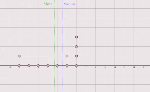
This example demonstrates the concepts of mean and median through dynamic graphics. It involves core statistical concepts and uses GeoGebra commands like Point and DynamicCoordinates to construct the graph. Suitable for middle school and above students to learn statistics and data analysis.
GeoGebra Commands & Parameters
Point(xAxis) → APoint(xAxis) → DPoint(xAxis) → CPoint(xAxis) → BPoint(xAxis) → EPoint(xAxis) → FPoint(xAxis) → GPoint(xAxis) → HPoint(xAxis) → IPoint(xAxis) → JPoint(xAxis) → KPoint(xAxis) → LDynamicCoordinates(A, x(A), CountIf[x(A) ≟ x(P), P, {B, C, D, E, F, G, H, I, J, K, L}]) → A_dDynamicCoordinates(B, x(B), CountIf[x(B) ≟ x(P), P, {C, D, E, F, G, H, I, J, K, L}]) → B_dDynamicCoordinates(C, x(C), CountIf[x(C) ≟ x(P), P, {D, E, F, G, H, I, J, K, L}]) → C_dDynamicCoordinates(D, x(D), CountIf[x(D) ≟ x(P), P, {E, F, G, H, I, J, K, L}]) → D_dDynamicCoordinates(E, x(E), CountIf[x(E) ≟ x(P), P, {F, G, H, I, J, K, L}]) → E_dDynamicCoordinates(F, x(F), CountIf[x(F) ≟ x(P), P, {G, H, I, J, K, L}]) → F_dDynamicCoordinates(G, x(G), CountIf[x(G) ≟ x(P), P, {H, I, J, K, L}]) → G_dDynamicCoordinates(H, x(H), CountIf[x(H) ≟ x(P), P, {I, J, K, L}]) → H_dDynamicCoordinates(I, x(I), CountIf[x(I) ≟ x(P), P, {J, K, L}]) → I_dDynamicCoordinates(J, x(J), CountIf[x(J) ≟ x(P), P, {K, L}]) → J_dDynamicCoordinates(K, x(K), CountIf[x(K) ≟ x(P), P, {L}]) → K_dDynamicCoordinates(L, x(L), 0) → L_d