
Epsilon-Delta Continuity Definition Demo by styler17
Loading the math board and drawing, please wait…
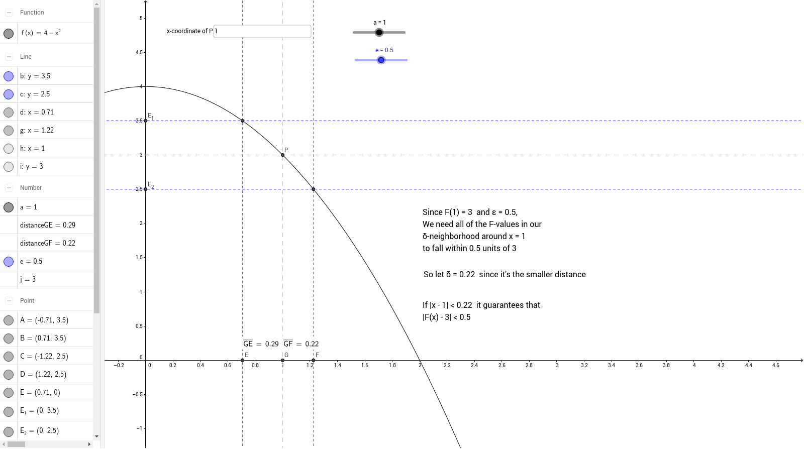
This example dynamically demonstrates the epsilon-delta definition of continuity, visually illustrating the geometric meaning of a function's continuity at a point. Key math concepts include continuity, epsilon-delta language, and function limits. It uses GeoGebra commands like Textfield, OrthogonalLine, Intersect, and Distance to construct function graphs, tangent lines, perpendicular lines, and distance calculations. Suitable for high school and above mathematics learners, especially beginners in calculus.
GeoGebra Commands & Parameters
Textfield(a) → inputBox1OrthogonalLine(E_1, yAxis) → bOrthogonalLine(E_2, yAxis) → cIntersect(f, b) → A, BIntersect(f, c) → C, DOrthogonalLine(B, xAxis) → dOrthogonalLine(D, xAxis) → gOrthogonalLine(P, xAxis) → hIntersect(xAxis, d) → EIntersect(xAxis, g) → FIntersect(xAxis, h) → GOrthogonalLine(P, yAxis) → iDistance(G, F) → distanceGFDistance(G, E) → distanceGE
AI Drawing Prompt Reference
Draw a function curve and illustrate the epsilon-delta definition of continuity at a point. Choose a fixed point on the curve, and draw a vertical line through it perpendicular to the x-axis, and a horizontal line perpendicular to the y-axis. On the y-axis, set two adjustable parameters representing epsilon and delta bounds, and draw horizontal lines through these points to intersect the function curve, yielding two pairs of intersection points. From these intersections, drop perpendiculars to the x-axis, marking the corresponding interval endpoints on the x-axis. Finally, measure and display the distances between these x-axis endpoints to show the epsilon-delta relationship.
The prompt above was compiled from the original drawing commands and is for reference only.