
Earth Model (cities, references, curves)
Loading the math board and drawing, please wait…
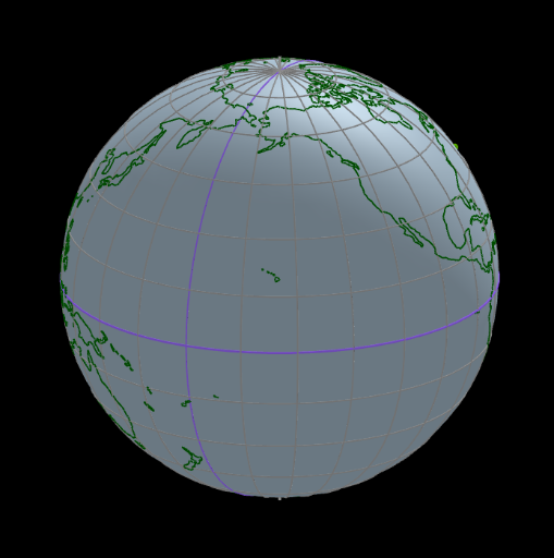
This example demonstrates an Earth model incorporating cities, reference lines, and curves. It involves core mathematical concepts such as spheres, coordinate geometry, vectors, parametric equations, and trigonometry. The construction utilizes GeoGebra commands and objects like Length, Element, Segment, Sequence, KeepIf, Sphere, PointIn, Ray, IntersectPath, Arc, Point, Center, Angle, Vector, Intersect, CircumcircleSector, Circle, OrthogonalPlane, Rotate, If, and CurveCartesian. Suitable for high school students and educators.
GeoGebra Commands & Parameters
Length(capitalesLista) → capitalesNumElement(tiempo, 7) → añoSegment(PS + (0.075 * PS), PN + (0.075 * PN)) → ejeLength(ciudadesLista) → ciudadesNumSequence(If[Element[ciudadesLista, k] > 0, k, 0], k, 1, ciudadesNum) → ciudadesElegidas1KeepIf(x > 0, ciudadesElegidas1) → ciudadesElegidas2Length(ciudadesElegidas2) → ciudadesNumElegidasSequence((5; Element[ciudadesLongitud, Element[ciudadesElegidas2, k]]°; Element[ciudadesLatitud, Element[ciudadesElegidas2, k]]°), k, 1, ciudadesNumElegidas) → ciudadesSequence((1.5 * Element[ciudades, k]), k, 1, ciudadesNumElegidas) → baseCiudadesSequence(Text[Element[ciudadesNombres, Element[ciudadesElegidas2, k]], Element[baseCiudades, k] + (0.03, 0.03, 0.03)], k, 1, ciudadesNumElegidas) → ciudadesNombresVisiblesSphere((0, 0, 0), (0.999 * 5)) → tierraPointIn(tierra) → ASequence(Segment[(0, 0, 0), Element[baseCiudades, k]], k, 1, ciudadesNumElegidas) → laserOtrosPointIn(tierra) → BRay(A, (2 * A)) → laserARay(B, (2 * B)) → laserBPointIn(tierra) → CIntersectPath(Plane[(0, 0, 0), A, B], tierra) → ortodromiaABArc(ortodromiaAB, A, B) → arcoOrtodromiaABSegment(PN, PS) → eje2Point(eje2) → LIntersectPath(Plane[L, A, B], tierra) → circuloLABCenter(circuloLAB) → DSegment(A, D) → segmentoDASegment(D, B) → segmentoDBArc(circuloLAB, A, B) → arcoCirculoLABRay(C, (2 * C)) → laserCIntersectPath(Plane[(0, 0, 0), A, C], tierra) → ortodromiaACIntersectPath(Plane[(0, 0, 0), B, C], tierra) → ortodromiaBCArc(ortodromiaAC, A, C) → arcoOrtodromiaACArc(ortodromiaBC, B, C) → arcoOrtodromiaBCAngle(A, (0, 0, 0), B) → angAOBAngle(A, (0, 0, 0), C) → angAOCAngle(B, (0, 0, 0), C) → angBOCVector((1; (-rot) + 180°; (-inclinacion))) → dirRay((0, 0, 0), Midpoint[A, A']) → gIntersect(g, tierra) → A'',CircumcircleSector(A, A'', A') → sectorLatitudARay((0, 0, 0), Midpoint[(5; 0; 0), A']) → hIntersect(h, tierra) → A''',CircumcircleSector((5; 0; 0), A''', A') → sectorLongitudACircle((0, 0, 0), 5, eje) → ecuador2Circle((5; 0; (-anguloPolar)), (5; 90°; (-anguloPolar)), (5; 180°; (-anguloPolar))) → antarticoCircle((5; 0; anguloPolar), (5; 90°; anguloPolar), (5; 180°; anguloPolar)) → articoCircle((5; 0; anguloEcliptica), (5; 90°; anguloEcliptica), (5; 180°; anguloEcliptica)) → cancerCircle((5; 0; (-anguloEcliptica)), (5; 90°; (-anguloEcliptica)), (5; 180°; (-anguloEcliptica))) → capricornioCircle((0, 0, 0), 5, eje) → ecuadorCircle(PN, (5; 0; 0), PS) → greenwichSequence(Circle[PN, (5; (15° * k); 0), PS], k, 1, 11) → meridianosSequence(Circle[(5; 0; (15° * k)), (5; 90°; (15° * k)), (5; 180°; (15° * k))], k, 1, 5) → paralelosNSequence(Circle[(5; 0; (-15° * k)), (5; 90°; (-15° * k)), (5; 180°; (-15° * k))], k, 1, 5) → paralelosSSegment((0, 0, 0), A) → segmentoOASegment((0, 0, 0), B) → segmentoOBSegment((0, 0, 0), (5; 0; 0)) → radioOrthogonalPlane(A, zAxis) → planoAIntersectPath(planoA, tierra) → paraleloASphere((0, 0, 0), 5) → esferaRay((0, 0, 0), Midpoint[A, B]) → fIntersect(f, tierra) → AB,CircumcircleSector(A, AB, B) → sectorOrtodromiaABSegment((0, 0, 0), C) → radioCSequence(If[Element[capitalesLista, k] > 0, k, 0], k, 1, capitalesNum) → capitalesElegidas1KeepIf(x > 0, capitalesElegidas1) → capitalesElegidas2Length(capitalesElegidas2) → capitalesNumElegidasSequence((5; Element[capitalesLongitud, Element[capitalesElegidas2, k]]°; Element[capitalesLatitud, Element[capitalesElegidas2, k]]°), k, 1, capitalesNumElegidas) → capitalesSequence((1.5 * Element[capitales, k]), k, 1, capitalesNumElegidas) → baseCapitalesSequence(Text[Element[capitalesNombres, Element[capitalesElegidas2, k]], Element[baseCapitales, k] + (0.03, 0.03, 0.03)], k, 1, capitalesNumElegidas) → capitalesNombresVisiblesSequence(Segment[(0, 0, 0), Element[baseCapitales, k]], k, 1, capitalesNumElegidas) → laserCapitalRotate(AA + (1, 0), lox, AA) → BBIf(abs(arg(BL) - arg(A)) ≤ 180°, arg(BL) - arg(A), arg(BL) - arg(A) < -180°, 360° + arg(BL) - arg(A), arg(BL) - arg(A) - 360°) → incCurveCartesian((5 * cos(t + λ) / cosh((q * t))), (5 * sin(t + λ) / cosh((q * t))), (5 * tanh((q * t))), t, (-20 * pi), (20 * pi)) → loxodromia
AI Drawing Prompt Reference
Draw an Earth model featuring multiple cities, reference lines, and curves. Start by creating a sphere to represent the Earth, then mark several cities on its surface and add name labels for each. Next, draw rays from the center of the sphere to the cities, highlighting the intersection points of these rays with the sphere. Finally, use these points to sketch two sinusoidal curves and an arc to illustrate the Earth's latitude and longitude features.
The prompt above was compiled from the original drawing commands and is for reference only.