
Dynamic Demonstration of Trigonometry and Locus
Loading the math board and drawing, please wait…
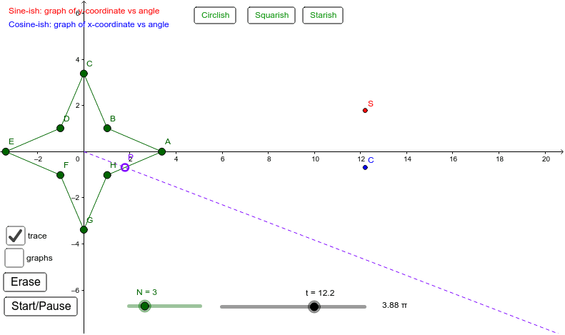
This example dynamically demonstrates the relationship between trigonometric functions and geometric shapes, particularly the locus of sine and cosine functions on the unit circle and their connection to triangles and line segments. The core math concepts involved include trigonometric functions, unit circle, locus, geometric construction, and analytical geometry. The construction utilizes GeoGebra commands such as Ray, Point, PolyLine, Intersect, and Locus. It is suitable for high school students learning trigonometry and analytical geometry to understand the dynamic relationship between function graphs and geometric figures.
GeoGebra Commands & Parameters
Ray((0, 0), Rotate[(1, 0), t]) → fPoint(xAxis) → A_1PolyLine(B, C, D, E, F, G, H, A, B) → gIntersect(f, g) → P, O_1, O_2Locus(K, t) → loc1Locus(L, t) → loc2
AI Drawing Prompt Reference
Draw a dynamic diagram illustrating the relationship between trigonometric functions and geometric shapes. Start with a unit circle centered at the origin. A ray from the origin rotates with an angle parameter, intersecting the circle. Place a moving point on the horizontal axis. Construct a closed polyline through several vertices, connecting them to form a geometric shape related to trigonometry. The ray intersects this polyline at multiple points, one of which moves as the angle changes. Two additional points trace loci as the angle varies, producing two curves that represent the sine and cosine functions. The overall figure shows how the angle on the unit circle corresponds to the function graphs.
The prompt above was compiled from the original drawing commands and is for reference only.