
Dynamic Demonstration of Cumulative Frequency and Boxplots
Loading the math board and drawing, please wait…
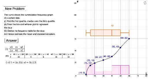
This example provides an interactive visualization of the transition from raw data distribution to cumulative frequency curves and boxplots. It covers essential statistical concepts including frequency distribution, cumulative frequency, medians, quartiles, and data dispersion. The construction leverages GeoGebra commands such as Random and Sequence for data generation, Sort for organizing values, Histogram for frequency visualization, and BoxPlot for summary statistics. A smooth cumulative frequency curve is rendered using the Spline command, while TableText and Join are used for structured data display. This tool is ideal for middle and high school students studying probability and statistics to intuitively grasp the relationship between data sets and their statistical representations.
GeoGebra Commands & Parameters
Random(5, 5) → n1Sequence(e1, e2, 10) → l3Sequence(((Element[l3, i] * "≤x<") * Element[l3, i + 1]), i, 1, n1) → l16Element(m1, a) → l1Spline(l2, 3) → bSequence(round(Intersect[x = Element[l3, i], b], 0), i, 1, n1 + 1) → l4IndexOf((0, 0), l4) → cRemove(l4, {(0, 0)}) → l5Sort(Unique[Join[{l2, l5}]]) → l6Spline(l6, 3) → dLength(l7) → fSequence(If[IsInteger[x(Element[l7, i]) / 10], Element[l7, i], (0, 0)], i, 1, f) → l8Sequence(y(Element[l9, i + 1]) - y(Element[l9, i]), i, 1, n1) → l10Histogram(l3, l10) → eSequence((Element[l3, i] + Element[l3, i + 1]) / 2, i, 1, n1) → l11mean(l11, l10) → m2TableText(l12, l13, "c|_ ") → text4Join({{"x"}, l16}) → l14Join({{"f"}, l10}) → l15TableText(l14, l15, "c|_ ") → text5BoxPlot(n + 10, 5, e1, q1, m, q3, e2) → gElement(l7, 2) → HElement(l7, 3) → IElement(l7, 4) → JElement(l7, 5) → KElement(l7, 6) → LElement(l7, 7) → MElement(l7, 1) → GElement(l7, 8) → NIf(e ≟ 600 ∨ e ≟ 800 ∨ e ≟ 1000, 1, 0) → h