
Draw Best Fit Line
Loading the math board and drawing, please wait…
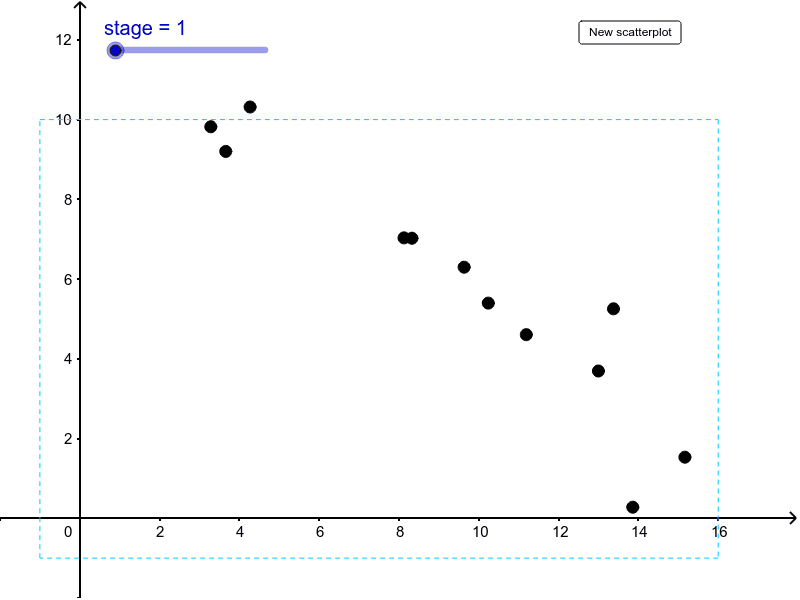
This example allows students to estimate the least squares regression line with visual aids. It covers key concepts in statistics, such as linear regression. Using GeoGebra commands like Random, Line, Polygon, Intersect, Point, Sequence, Zip, FitLineY, Sum, PMCC, students can understand how to construct the best fit line. Suitable for high school and above students learning linear regression and statistical analysis.
GeoGebra Commands & Parameters
Random(0, 1) → list3Line(If[Element[list2, 1] ≟ 1, (0, list3 * 5 + RandomUniform[0, 5]), (RandomUniform[0, 8], list3 * 10)], If[Element[list2, 2] ≟ 1, (16, 5 * (1 - list3) + RandomUniform[0, 5]), (8 + RandomUniform[0, 8], 10 - 10 * list3)]) → fPolygon((-1, -1), (-1, 10), (16, 10), (16, -1)) → poly1, b, c, d, eIntersect(f, poly1) → F, GPoint(poly1) → DPoint(poly1) → ELine(D, E) → gSequence(RandomUniform[x(F) + n, x(G)], t, 1, Random[8, 17]) → list1Zip((A, Slope[f] * A + y(Intersect[f, yAxis]) + RandomUniform[-Random[0, 3] + n, RandomUniform[0, 3]]), A, list1) → list4FitLineY(list4) → hZip((x(A), x(A) * Slope[g] + y(Intersect[g, yAxis])), A, list4) → list5Zip(Segment[A, B], A, list4, B, list5) → list6Zip(Polygon[A, B, 4], A, list4, B, list5) → list7Sum(Zip[Polygon[B, (A, Slope[h] * A + y(Intersect[h, yAxis])), 4], A, list1, B, list4]) → list8PMCC(list4) → r
AI Drawing Prompt Reference
Draw a best fit line by first generating some random points, then drawing a line through these points. Use these points and the line to estimate the best fit line, and draw segments between the original line and the best fit line. Finally, calculate the correlation coefficient of these points.
The prompt above was compiled from the original drawing commands and is for reference only.