
Dividing Fractions Visual Model
Loading the math board and drawing, please wait…
In collections
Fraction worksheets
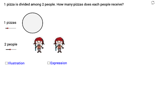
This example demonstrates a visual model for dividing fractions. Key mathematical concepts include fraction division. Using GeoGebra commands such as Point, Segment, Sequence, and Polygon, the process of fraction division is clearly illustrated. Suitable for high-grade elementary or junior high school students learning fraction division.
GeoGebra Commands & Parameters
Point(Segment[(x(D) + 2 / 5, y(D)), (x(D) + 1, y(D))]) → SSegment(A, (x(A) + 1, y(A))) → l1Point(Segment[(x(A) + 1 / 5, y(A)), (x(A) + 1, y(A))]) → PSegment(B, (x(B) + 1, y(B))) → l2Point(Segment[(x(B) + 2 / 6, y(B)), (x(B) + 1, y(B))]) → QPoint(Segment[(x(C) + 1 / 6 - 0.005, y(C)), (x(Q) - 1 / 6, y(C))]) → RSegment(C, (x(C) + 1, y(C))) → l3Sequence(Circle[((2.5 * (i - 1)), 0), 1], i, 1, a) → list1Sequence(Segment[((2.5 * a), 0), ((2.5 * a) - sin((j * θ)), cos((j * θ)))], j, 1, c - 1) → list2Segment(D, (x(D) + 1, y(D))) → l4Polygon((0.016528925619834656, -3), (1.2165289256198346, -3), (1.2165289256198346, -1.3), (0.016528925619834656, -1.3)) → poly1, e, g, h, iGCD(a, d) → kSegment(A, P) → jSegment(C, R) → lSegment(B, Q) → mSegment(D, S) → nPoint(Segment[(x(A_1) + 1 / 7, y(A_1)), (x(A_1) + 1, y(A_1))]) → P_1Segment(A_1, P_1) → j_1Point(Segment[(x(D_1) + 2 / 5, y(D_1)), (x(D_1) + 1, y(D_1))]) → S_1Point(Segment[(x(A_2) + 1 / 7, y(A_2)), (x(A_2) + 1, y(A_2))]) → P_2GCD(a_1, d_1) → k_1Segment(A_2, P_2) → j_2Segment(D_1, S_1) → n_1Point(Segment[(x(D_2) + 2 / 5, y(D_2)), (x(D_2) + 1, y(D_2))]) → S_2Point(Segment[(x(A_3) + 1 / 7, y(A_3)), (x(A_3) + 1, y(A_3))]) → P_3GCD(a_2, d_2) → k_2Segment(A_3, P_3) → j_3Segment(D_2, S_2) → n_2Sequence(Sequence[CircleSector[(((-f) * sin((((2 * k) - 1) * θ / 2))) + (2.5 * (m - 1)), (f * cos((((2 * k) - 1) * θ / 2)))), (((-f) * sin((((2 * k) - 1) * θ / 2))) - sin(((k - 1) * θ)) + (2.5 * (m - 1)), (f * cos((((2 * k) - 1) * θ / 2))) + cos(((k - 1) * θ))), (((-f) * sin((((2 * k) - 1) * θ / 2))) - sin((k * θ)) + (2.5 * (m - 1)), (f * cos((((2 * k) - 1) * θ / 2))) + cos((k * θ)))], k, 1, 1], m, 1, a) → list4Sequence(Sequence[CircleSector[((f * sin((((2 * k) - 1) * θ / 2))) + (2.5 * (m - 1)), (f * cos((((2 * k) - 1) * θ / 2)))), ((f * sin((((2 * k) - 1) * θ / 2))) + sin((k * θ)) + (2.5 * (m - 1)), (f * cos((((2 * k) - 1) * θ / 2))) + cos((k * θ))), ((f * sin((((2 * k) - 1) * θ / 2))) + sin(((k - 1) * θ)) + (2.5 * (m - 1)), (f * cos((((2 * k) - 1) * θ / 2))) + cos(((k - 1) * θ)))], k, 1, b], m, 1, a) → list3
AI Drawing Prompt Reference
Draw a visual model for fraction division. Start by drawing the lengths of the denominators of two fractions, then draw the lengths of the numerators. Next, mark the division points on the denominators and numerators, and connect these points with line segments. Finally, draw a quadrilateral to represent the fraction division process. Use points, line segments, sequences, and polygons to ensure the model clearly illustrates the fraction division process.
The prompt above was compiled from the original drawing commands and is for reference only.