
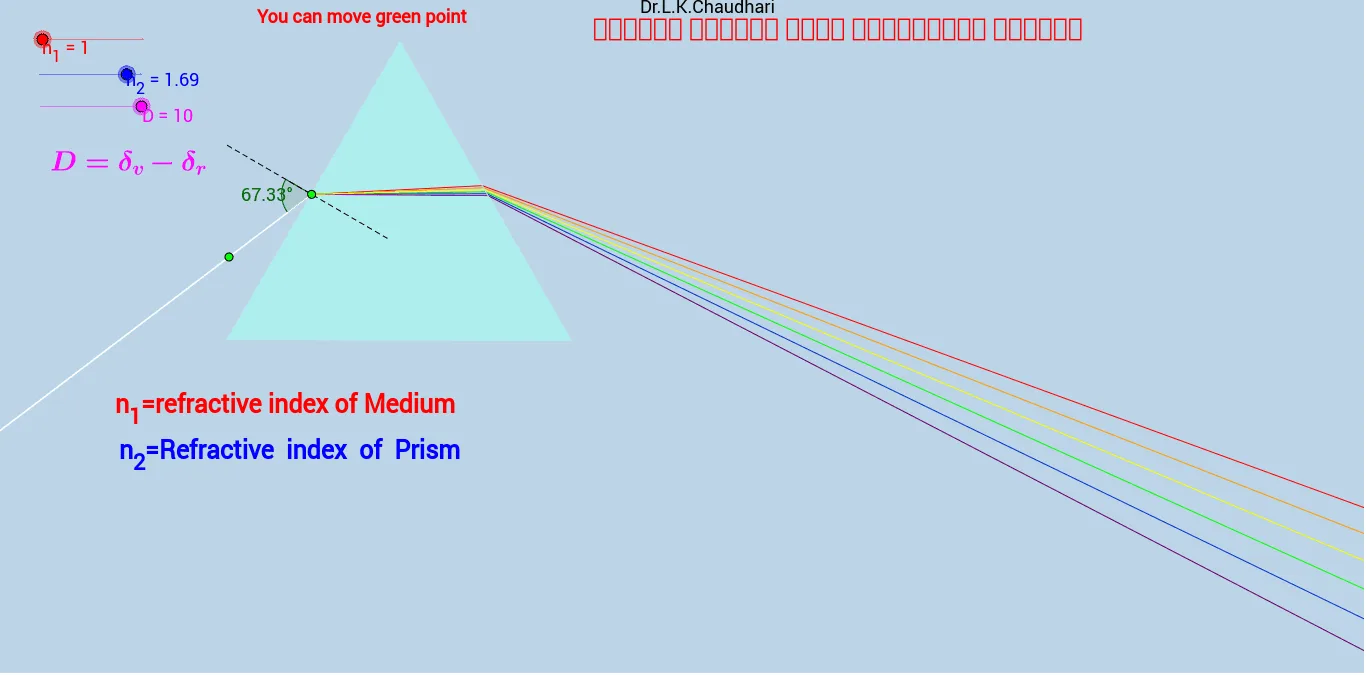
Dispersion of White Light by a Prism (Geometric Simulation)
Loading the math board and drawing, please wait…
① This GeoGebra example simulates the dispersion of white light through a triangular prism, visually demonstrating how different colors separate due to varying refractive indices along geometric paths. ② Core mathematical concepts include basic geometric elements such as points, polygons, angles, straight lines, slopes, perpendiculars, rotations, intersections, and segments, along with trigonometric functions used in angle calculations; it also integrates physical optics principles of refraction and dispersion into a geometric construction. ③ Construction highlights: Based on the summary, the example employs GeoGebra commands like Point, Polygon, OrthogonalLine, Angle, Ray, Slope, Rotate, Intersect, and Segment to build the prism polygon (poly1), incident and refracted rays, normals, and multiple auxiliary points (D, B, A, C, E, F, G, etc.), with angles α, β, γ, δ controlling ray directions and intersections/segments completing the light path. ④ Suitable for middle or high school physics/math classes explaining refraction, dispersion, and geometric construction, as well as introductory university optics or geometric modeling, helping students understand how geometric tools can simulate physical phenomena.
GeoGebra Commands & Parameters
Point(xAxis) → APolygon(A, B, 3) → poly1, c, a, b, CPoint(b) → D_2OrthogonalLine(D_2, b) → ePoint(e) → FPoint(e) → GAngle(F, D_2, E) → αRay(D_2, E) → dSlope(d) → mRotate(G, asin((n_1 / n_2 * sin(α))), D_2) → G'Ray(D_2, G') → fIntersect(a, f) → HSegment(H, D_2) → gOrthogonalLine(H, a) → hPoint(h) → IAngle(D_2, H, I) → γPoint(h) → JRotate(J, (-asin((n_2 / n_1 * sin(γ)))), H) → J'Angle(J', H, J) → δRay(H, J') → iSegment(F, G) → jSegment(J, I) → kAngle(G, D_2, G') → βRotate(G, asin((n_1 / (((1 + (0.002 * D)) * n_2)) * sin(α))), D_2) → PRotate(G, asin((n_1 / (((1 + (0.004 * D)) * n_2)) * sin(α))), D_2) → QRotate(G, asin((n_1 / (((1 + (0.006 * D)) * n_2)) * sin(α))), D_2) → RRotate(G, asin((n_1 / (((1 + (0.008 * D)) * n_2)) * sin(α))), D_2) → SRay(D_2, P) → sRay(D_2, Q) → tRay(D_2, R) → a_1Ray(D_2, S) → b_1Rotate(G, asin((n_1 / (((1 + (0.01 * D)) * n_2)) * sin(α))), D_2) → TRay(D_2, T) → c_1Intersect(a, s) → UIntersect(a, a_1) → VIntersect(a, t) → WIntersect(a, b_1) → ZIntersect(a, c_1) → A_1OrthogonalLine(U, a) → d_1OrthogonalLine(W, a) → e_1OrthogonalLine(V, a) → f_1OrthogonalLine(Z, a) → i_1OrthogonalLine(A_1, a) → l_1Point(d_1) → B_1Point(e_1) → C_1Point(f_1) → D_1Point(i_1) → E_1Point(l_1) → F_1Rotate(B_1, (-asin((((1 + (0.002 * D)) * n_2 / n_1) * sin(γ)))), U) → G_1Rotate(C_1, (-asin((((1 + (0.004 * D)) * n_2 / n_1) * sin(γ)))), W) → H_1Rotate(D_1, (-asin((((1 + (0.006 * D)) * n_2 / n_1) * sin(γ)))), V) → I_1Rotate(E_1, (-asin((((1 + (0.008 * D)) * n_2 / n_1) * sin(γ)))), Z) → J_1Rotate(F_1, (-asin((((1 + (0.01 * D)) * n_2 / n_1) * sin(γ)))), A_1) → K_1Ray(U, G_1) → nRay(W, H_1) → pRay(V, I_1) → qRay(Z, J_1) → rRay(A_1, K_1) → lSegment(D_2, U) → g_1Segment(D_2, V) → h_1Segment(D_2, Z) → j_1Segment(D_2, A_1) → k_1Segment(D_2, W) → m_1Intersect(b, a) → KIntersect(b, c) → LIntersect(a, c) → MPolygon(K, L, M) → poly2, m_2, k_2, l_2