
Disc Method for Volume of Solids of Revolution
Loading the math board and drawing, please wait…
In collections
volume of revolution
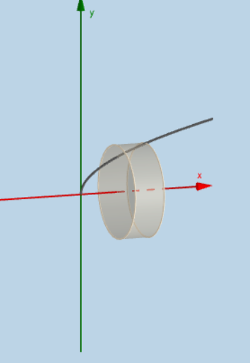
This example demonstrates the calculation of volumes of solids of revolution using the disc method. It involves core calculus concepts such as integration, rotation of function graphs, and volume computation. Key GeoGebra commands used include Sequence, Rotate, Intersect, Polygon, Circle, Surface, Cylinder, Dilate, Segment, Textfield, and Integral. Suitable for high school students and above, or anyone learning calculus, to visualize and understand the volume calculation process of rotational solids.
GeoGebra Commands & Parameters
Sequence(Polygon[(a + (i * deltax), 0), (a + ((i + 1) * deltax), 0), (a + ((i + 1) * deltax), f(a + ((i + 1) * deltax))), (a + (i * deltax), f(a + ((i + 1) * deltax)))], i, 0, n - 1, 1) → list1Rotate(list1, α, y = 0) → list1'Intersect(i, l) → BIntersect(k, l) → CIntersect(j, k) → DPolygon(C, B, A, D) → poly1, c_2, b_1, a_1, dRotate(C, α, y = 0) → C'Rotate(B, α, y = 0) → B'Rotate(A, α, y = 0) → A'Rotate(D, α, y = 0) → D'Polygon(C', B', A', D') → poly1', c', b', a', d'Sequence((a + (i * deltax), 0), i, 0, n, 1) → list2Sequence((a + (i * deltax), f(a + (i * deltax))), i, 1, n, 1) → list3Rotate(list3, α, y = 0) → list3'Sequence((a + (i * deltax), f(a + ((i + 1) * deltax))), i, 0, n - 1, 1) → list4Sequence(x = a + (i * deltax), i, 1, n, 1) → list6Sequence(Segment[Element[list3, i], Element[list4, i]], i, 0, n, 1) → list5Sequence(CircleSector[Element[list2, i + 1], Element[list3', i], Element[list3, i], xOyPlane], i, 1, n, 1) → list7Sequence(Cylinder[Element[list2, i], Element[list2, i + 1], f(Element[list2, i + 1])], i, 1, n, 1) → list8Sequence(Circle[Element[list2, i], f(Element[list2, i]), x = 0], i, 2, n + 1, 1) → list10Circle((a, 0), f(a + deltax), x = 0) → pSurface(q, α) → eCylinder((x(A), 0), (x(A) - deltax, 0), y(A)) → o, r, s, tDilate(E, If[0 < u ≤ 1, 1 - u, 0], D) → E'Dilate(F, If[0 < u ≤ 1, 1 - u, 0], A) → F'Segment(E, E') → f_1Segment(F, F') → g_1Dilate(D, If[1 < u ≤ 2, 2 - u, 0], A) → D'_1Segment(D, D'_1) → h_1Rotate(F, α, y = 0) → F'_1Rotate(F', α, y = 0) → F''Segment(F'_1, F'') → i_1Rotate(E, α, y = 0) → E'_1Rotate(E', α, y = 0) → E''Segment(E'_1, E'') → j_1Rotate(D, α, y = 0) → D'_2Rotate(D'_1, α, y = 0) → GSegment(D'_2, G) → k_1Textfield(f) → InputBox1Textfield(a) → InputBox2Textfield(b) → InputBox3Integral(f, a, b) → m_1
AI Drawing Prompt Reference
Visualize the calculation of volumes of solids of revolution using the disc method. Start by drawing a function graph and dividing it into small rectangles. Rotate these rectangles to form a series of discs, which combine to create the solid of revolution. Show the integration process to compute the volume, labeling key points and rotation angles to clearly illustrate the transformation from rectangles to discs to the final solid.
The prompt above was compiled from the original drawing commands and is for reference only.