
Disc Method Demonstration by jameshammer3
Loading the math board and drawing, please wait…
In collections
Volumes of Solids
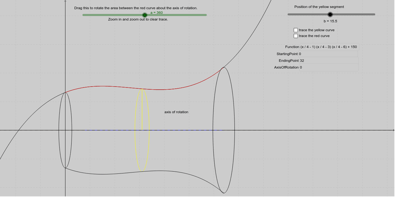
This example dynamically demonstrates the disc method for calculating the volume of a solid of revolution. It involves core math concepts like integration, function graphing, and volume calculation of rotated bodies. Constructed using GeoGebra commands such as Intersect, Segment, CurveCartesian, Textfield, and Function. Suitable for high school students and above learning calculus volume methods or for educational presentations.
GeoGebra Commands & Parameters
Intersect(h, f, (-9.415320057953506, 4.177991286269389E-12)) → ASegment((b, h(b)), (b, f(b))) → jCurveCartesian(t + (f(t) - m) * sin(a°) / 100, m + (f(t) - m) * cos(a°), t, 4, 32) → gCurveCartesian(b + (f(b) - m) * sin(t°) / 100, m + (f(b) - m) * cos(t°), t, 0, a) → kCurveCartesian(b + (h(b) - m) * sin(t°) / 100, m + (h(b) - m) * cos(t°), t, 0, a) → lSegment((b + (h(b) - m) * sin(a°) / 100, m + (h(b) - m) * cos(a°)), (b + (f(b) - m) * sin(a°) / 100, m + (f(b) - m) * cos(a°))) → iCurveCartesian(t + (f(t) - m) * sin(a°) / 100, m + (f(t) - m) * cos(a°), t, 4, 32) → qCurveCartesian(b + (f(b) - m) * sin(t°) / 100, m + (f(b) - m) * cos(t°), t, 0, a) → sCurveCartesian(b + (h(b) - m) * sin(t°) / 100, m + (h(b) - m) * cos(t°), t, 0, a) → uTextfield(initial) → inputBox1CurveCartesian(initial + (h(initial) - m) * sin(t°) / 100, m + (h(initial) - m) * cos(t°), t, 0, a) → dTextfield(terminal) → inputBox2CurveCartesian(t + (h(t) - m) * sin(a°) / 100, m + (h(t) - m) * cos(a°), t, initial, terminal) → cTextfield(h) → inputBox3Textfield(m) → inputBox4CurveCartesian(t + (h(t) - m) * sin(a°) / 100, m + (h(t) - m) * cos(a°), t, initial, terminal) → oCurveCartesian(terminal + (h(terminal) - m) * sin(t°) / 100, m + (h(terminal) - m) * cos(t°), t, 0, a) → eFunction(-h(x) + 2 * m, initial, terminal) → g_1
AI Drawing Prompt Reference
Draw a function curve and its rotated solid of revolution to demonstrate the disc method for volume calculation. Start by plotting the function and a horizontal line, marking their intersection. Draw vertical segments from the intersection point and the endpoints of the function curve down to the horizontal line. Then, sketch the cross-section of the solid, including two circles and a connecting segment. Add text boxes to input the function and rotation angle, and use curves to dynamically show the rotation process and the integral area.
The prompt above was compiled from the original drawing commands and is for reference only.