
Differential Equations Visualization
Loading the math board and drawing, please wait…
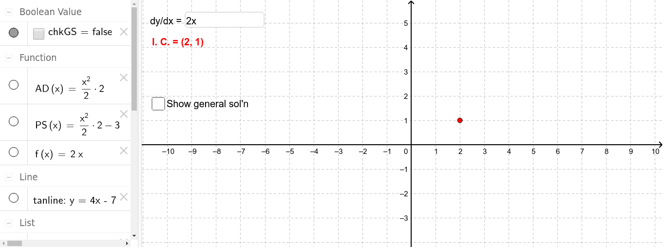
This example dynamically demonstrates the solution and geometric meaning of differential equations using GeoGebra, ① visually showing the relationship between integral curves and tangent lines of differential equations; ② involving core concepts: differential equations, derivatives, integrals, tangent lines, confidence intervals, random variables; ③ construction highlights: using commands like Integral, Textfield, Tangent, Slope, Sequence and objects f, AD, IC, inpF, C, PS, tanline, m, txtIC, txtSlope, GS, chkGS, txtSoln; ④ suitable for high school students and mathematics enthusiasts learning calculus and equation applications.
GeoGebra Commands & Parameters
Integral(f) → ADTextfield(f) → inpFTangent(IC, PS) → tanlineSlope(tanline) → mSequence(AD(x) + i, i, -20, 20, 1) → GS
AI Drawing Prompt Reference
Create a dynamic visualization showing the solution and geometric meaning of differential equations, illustrating the relationship between integral curves and tangent lines, including function graphs, tangent lines, integral curves, and random variables, start by plotting the function, then draw tangent lines and integral curves on it, connect them with dashed lines, and label the function expression and slope of the tangent lines.
The prompt above was compiled from the original drawing commands and is for reference only.