
Differential Equation Graph
Loading the math board and drawing, please wait…
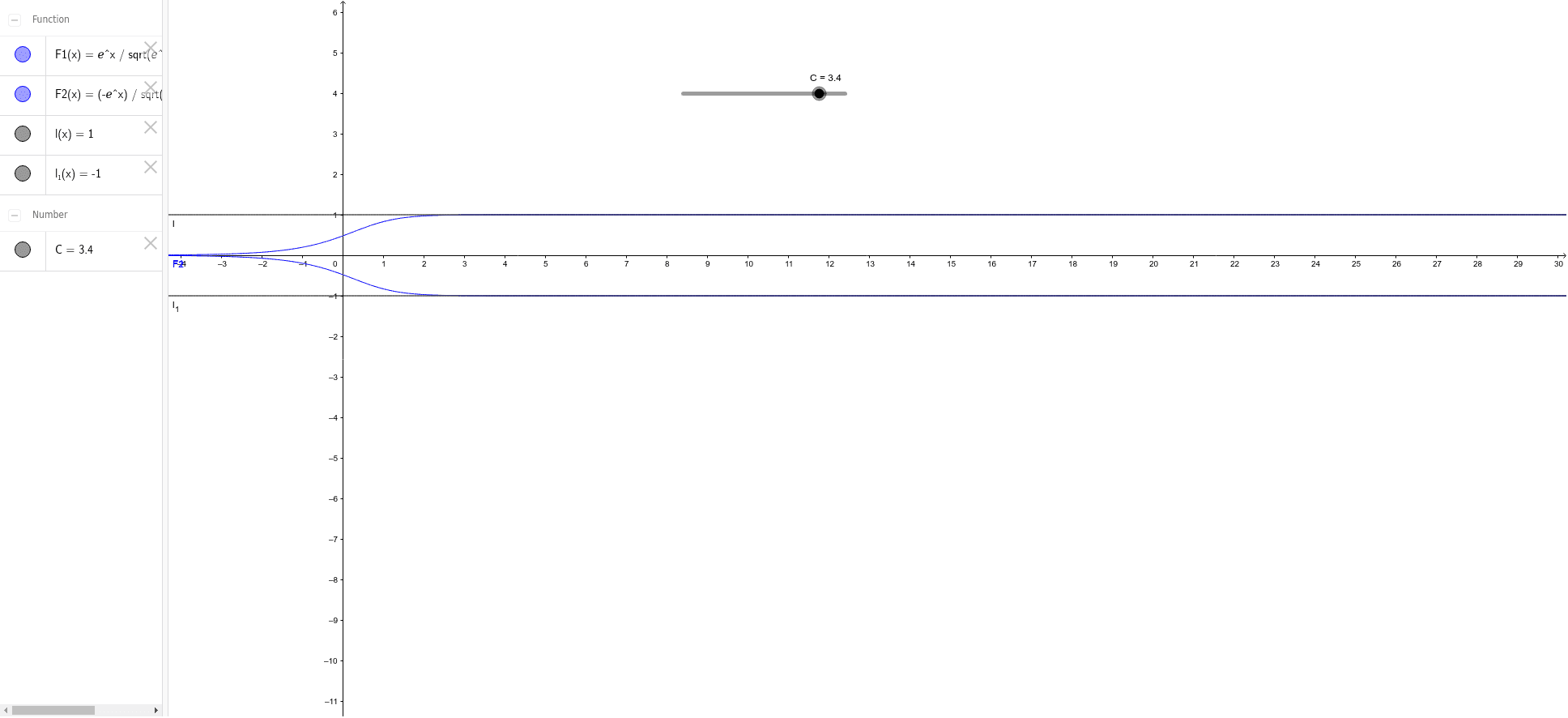
This example demonstrates the graph of a differential equation. It involves core concepts in calculus, particularly derivatives and integrals. Using GeoGebra commands such as C, F1, F2, l, l_1, one can dynamically observe how the solutions of differential equations change. Suitable for university-level calculus and ordinary differential equations courses.
GeoGebra Commands & Parameters
Numeric C(3.4)F1(x) = ℯ^(x) / sqrt(ℯ^((2 * x)) + C)F2(x) = ((-ℯ^(x))) / sqrt(ℯ^((2 * x)) + C)l(x) = 1l_1(x) = -1
AI Drawing Prompt Reference
Draw a graph featuring two exponential functions symmetric about the x-axis, with their expressions involving a constant C, and include two horizontal reference lines y=1 and y=-1 to illustrate the relationship between the solutions of the differential equation and the reference lines, suitable for university-level calculus and ODE courses.
The prompt above was compiled from the original drawing commands and is for reference only.