Dice Rolling Probability Demo

Loading the math board and drawing, please wait…

2015-02-06 17:56

In collections Statistics & Probability Simulations of Coins and Dice probability simulations

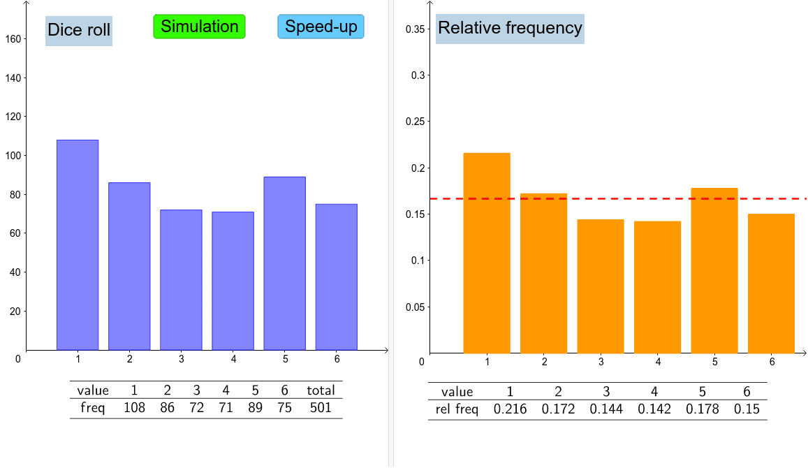
This example demonstrates dice rolling probability distribution and expected value calculation. It involves core math concepts like matrices, cylinders, probability distributions, and circles. Construction highlights include commands and objects such as Unique, Frequency, Sum, Random, BarChart, Ray, Append, TableText. Suitable for high school mathematics teaching, particularly for probability statistics and geometry integration cases.

GeoGebra Commands & Parameters

Unique(dlist) → list1
Frequency(dlist) → dfreq
Sum(dfreq) → sum
Random(1, 6) → dice1
BarChart(dlist, 0.8) → b
Ray((0, 0.16666666666666666), (7, 0.16666666666666666)) → d
Append("freq", dfreq) → row2
Append("value", list1) → row1
Append("rel freq", relfreq) → row3
Append(row1, "total") → row1a
Append(row2, sum) → row2a
TableText({row1a, row2a}, "c_") → text2
TableText({row1, row3}, "c_") → text3
BarChart(list1, relfreq, 0.8) → a

AI Drawing Prompt Reference

Create a visualization demonstrating dice rolling probability distribution and expected value calculation, incorporating core mathematical concepts like matrices, cylinders, probability distributions, and circles. Start by plotting a bar chart to represent the frequency of each dice roll. Add a ray as an axis. Then, use a table to display the numbers, frequencies, and relative frequencies, summarizing them into a total table. Finally, plot another bar chart showing the correspondence between numbers and relative frequencies.

The prompt above was compiled from the original drawing commands and is for reference only.