
Definite Integral Illustrator (II)
Loading the math board and drawing, please wait…
This example demonstrates how to use GeoGebra to visualize definite integrals, including left sum, right sum, and midpoint sum methods. Core math concepts involve definite integrals, inequalities, function graphs, triangles, and box plots. Construction highlights the use of commands and objects like Textfield, Sequence, Translate, LeftSum, Sum, Intersect, Polygon, Integral, etc., to show approximations of integral values through slider animations for different partition methods. Suitable for high school and early university students learning calculus and numerical integration concepts.
GeoGebra Commands & Parameters
Textfield(f) → InputBox1Textfield(a) → InputBox2Textfield(b) → InputBox3Sequence((a + (i * deltax), 0), i, 1, n, 1) → rightxSequence((a + (i * deltax), f(a + (i * deltax))), i, 1, n, 1) → fofrightxSequence((a + (i * deltax), 0), i, 0, n - 1, 1) → leftxSequence(Midpoint[Element[leftx, i], Element[rightx, i]], i, 1, n, 1) → midpointsSequence((a + (i * deltax), f(a + (i * deltax))), i, 1, n, 1) → list1Translate(list1, (deltax, 0)) → list1'LeftSum(f, a, b, n) → lSequence(x = x(Element[midpoints, i]), i, 1, n, 1) → list2Sequence(Intersect[f, Element[list2, i], (1.25, 1.118033988749895)], i, 1, n, 1) → list3Translate(list3, (deltax / 2, 0)) → midpointtoprightTranslate(list3, (((-deltax)) / 2, 0)) → midpointtopleftTranslate(midpoints, (deltax / 2, 0)) → midpoints'Translate(midpoints, (((-deltax)) / 2, 0)) → midpoints'_1Sequence(Polygon[Element[midpoints'_1, i], Element[midpoints', i], Element[midpointtopright, i], Element[midpointtopleft, i]], i, 1, n, 1) → list4Sum(list4) → hTranslate(list1, ((-deltax), 0)) → list1'_1Translate(rightx, ((-deltax), 0)) → rightx'Sequence(Polygon[Element[rightx, i], Element[list1, i], Element[list1'_1, i], Element[rightx', i]], i, 1, n, 1) → rightrectanglesumSum(rightrectanglesum) → jIntersect(k, p) → FIntersect(m, k) → GPolygon(D, E, G, F) → poly1, d_1, e, g_1, f_1Intersect(m, q) → HIntersect(p, q) → IPolygon(D, E, H, I) → poly2, d_2, e_1, h_1, i_1Intersect(p, r) → JIntersect(r, m) → KPolygon(D, E, K, J) → poly3, d_3, e_2, k_1, j_1Integral(f, a, b) → sSequence(Polygon[(a + (i * deltax), 0), (a + ((i + 1) * deltax), 0), (a + ((i + 1) * deltax), f(a + ((i + 1) * deltax))), (a + (i * deltax), f(a + (i * deltax)))], i, 0, n - 1, 1) → list5Sum(list5) → u
AI Drawing Prompt Reference
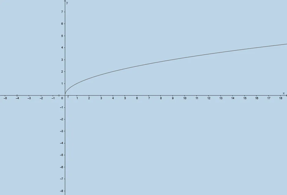
Draw the graph of the function y=f(x) in a coordinate plane and focus on the definite integral over the interval [a,b]. Using a chosen partition number n, construct three Riemann-sum visualizations: left-endpoint rectangles, right-endpoint rectangles, and midpoint rectangles. For each subinterval, place the rectangle bases on the x-axis and determine their top edges by intersecting vertical sides with the function. Arrange the three sets of rectangles so they clearly align over the same interval, separated slightly by horizontal shifts for visibility. Finally, indicate the definite integral from x=a to x=b beneath the curve as the target area representation.
The prompt above was compiled from the original drawing commands and is for reference only.