
Definite Integral Approximations
Loading the math board and drawing, please wait…
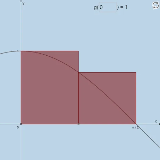
This example demonstrates the approximation of definite integrals using left endpoint, right endpoint, midpoint, and trapezoidal methods. It involves core math concepts like definite integrals, function graphs, rectangles, trapezoids, and geometric constructions. GeoGebra commands and objects such as Textfield, Sequence, Translate, LeftSum, Sum, Intersect, Polygon, Integral are used in the construction. Suitable for high school and above students learning about integral approximation techniques in calculus.
GeoGebra Commands & Parameters
Textfield(f) → InputBox1Textfield(a) → InputBox2Textfield(b) → InputBox3Sequence((a + (i * deltax), 0), i, 1, n, 1) → rightxSequence((a + (i * deltax), f(a + (i * deltax))), i, 1, n, 1) → fofrightxSequence((a + (i * deltax), 0), i, 0, n - 1, 1) → leftxSequence(Midpoint[Element[leftx, i], Element[rightx, i]], i, 1, n, 1) → midpointsSequence((a + (i * deltax), f(a + (i * deltax))), i, 1, n, 1) → list1Translate(list1, (deltax, 0)) → list1'LeftSum(f, a, b, n) → lSequence(x = x(Element[midpoints, i]), i, 1, n, 1) → list2Sequence(Intersect[f, Element[list2, i], (1.1780972450961724, 0.38268343236508984)], i, 1, n, 1) → list3Translate(list3, (deltax / 2, 0)) → midpointtoprightTranslate(list3, (((-deltax)) / 2, 0)) → midpointtopleftTranslate(midpoints, (deltax / 2, 0)) → midpoints'Translate(midpoints, (((-deltax)) / 2, 0)) → midpoints'_1Sequence(Polygon[Element[midpoints'_1, i], Element[midpoints', i], Element[midpointtopright, i], Element[midpointtopleft, i]], i, 1, n, 1) → list4Sum(list4) → hTranslate(list1, ((-deltax), 0)) → list1'_1Translate(rightx, ((-deltax), 0)) → rightx'Sequence(Polygon[Element[rightx, i], Element[list1, i], Element[list1'_1, i], Element[rightx', i]], i, 1, n, 1) → rightrectanglesumSum(rightrectanglesum) → jIntersect(k, p) → FIntersect(m, k) → GPolygon(D, E, G, F) → poly1, d_1, e, g_1, f_1Intersect(m, q) → HIntersect(p, q) → IPolygon(D, E, H, I) → poly2, d_2, e_1, h_1, i_1Intersect(p, r) → JIntersect(r, m) → KPolygon(D, E, K, J) → poly3, d_3, e_2, k_1, j_1Integral(f, a, b) → sSequence(Polygon[(a + (i * deltax), 0), (a + ((i + 1) * deltax), 0), (a + ((i + 1) * deltax), f(a + ((i + 1) * deltax))), (a + (i * deltax), f(a + (i * deltax)))], i, 0, n - 1, 1) → list5Sum(list5) → uTextfield(x_o) → InputBox4
AI Drawing Prompt Reference
Draw a function graph and show the approximation of definite integrals using left endpoint, right endpoint, midpoint, and trapezoidal methods. First, plot the function curve and the x-axis, then use rectangles and trapezoids to represent different approximation methods below the curve, labeling the calculation results of each method and the exact integral value. Start with the left endpoint method, then show the right endpoint, midpoint, and trapezoidal methods in sequence, distinguishing each with different colors and indicating the number of divisions and the area of each small region.
The prompt above was compiled from the original drawing commands and is for reference only.