Damped Harmonic Oscillator by robdjeff

Loading the math board and drawing, please wait…

2014-02-27 18:05

In collections Differential Equations

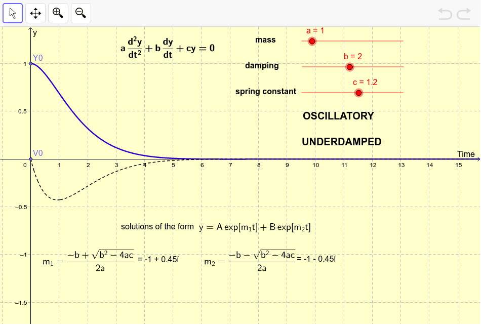
This example graphically demonstrates the solutions of homogeneous second-order differential equations, specifically the damped harmonic oscillator. It involves core mathematical concepts such as differential equations, vibration, damping, and frequency. The construction utilizes GeoGebra commands and objects like Point, If, and various parameters (c, V0, b, a, alpha2, alpha1, Y0, A_3, m2a, m1a, A_1, B_1, text elements, etc.) to illustrate the behavior of the system. It is suitable for high school students and above studying differential equations and physical vibration phenomena, as well as for university-level introductory physics instruction.

GeoGebra Commands & Parameters

Point(yAxis) → V0
Point(yAxis) → Y0
If(b^(2) > ((4 * a) * c), h''(x), If[b^(2) ≟ ((4 * a) * c), g''(x), f''(x)]) → acc
If(a ≟ 0, p'(x), If[b^(2) > ((4 * a) * c), h'(x), If[b^(2) ≟ ((4 * a) * c), g'(x), f'(x)]]) → v

AI Drawing Prompt Reference

Create a diagram of a damped harmonic oscillator illustrating solutions to a homogeneous second-order differential equation. Place two draggable points on the vertical axis representing initial displacement and initial velocity. Based on system parameters (mass, damping coefficient, stiffness), determine the damping type: overdamped, critically damped, or underdamped, and select the corresponding displacement curve. Also display velocity and acceleration curves derived from the displacement. Curves should be smooth and continuous, with key parameters like damping ratio and natural frequency labeled. The figure should clearly show oscillatory decay or critical return to equilibrium.

The prompt above was compiled from the original drawing commands and is for reference only.