
Cubic Surface Fitting
Loading the math board and drawing, please wait…
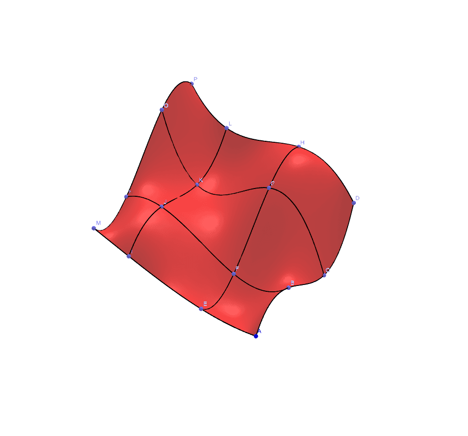
This example demonstrates how to perform cubic surface fitting using GeoGebra, illustrating the relationship between data and the fitted surface. Key math concepts include surface fitting, polynomial regression, and coefficient analysis. Construction highlights involve commands like PointIn, Point, Sequence, FitPoly, Coefficients, Surface, and CurveCartesian for creating data points, fitting surfaces, and displaying coefficients. Suitable for high school and above students learning data fitting, polynomial functions, and 3D graphing.
GeoGebra Commands & Parameters
PointIn(Plane[A, Plane[xAxis, zAxis]]) → BPointIn(Plane[A, Plane[xAxis, zAxis]]) → CPointIn(Plane[A, Plane[xAxis, zAxis]]) → DPointIn(Plane[A, Plane[yAxis, zAxis]]) → EPoint(IntersectPath[Plane[B, Plane[yAxis, zAxis]], Plane[E, Plane[xAxis, zAxis]]]) → FPoint(IntersectPath[Plane[C, Plane[yAxis, zAxis]], Plane[E, Plane[xAxis, zAxis]]]) → GPoint(IntersectPath[Plane[D, Plane[yAxis, zAxis]], Plane[E, Plane[xAxis, zAxis]]]) → HPointIn(Plane[A, Plane[yAxis, zAxis]]) → IPointIn(Plane[A, Plane[yAxis, zAxis]]) → MPoint(IntersectPath[Plane[B, Plane[yAxis, zAxis]], Plane[I, Plane[xAxis, zAxis]]]) → JPoint(IntersectPath[Plane[C, Plane[yAxis, zAxis]], Plane[I, Plane[xAxis, zAxis]]]) → KPoint(IntersectPath[Plane[D, Plane[yAxis, zAxis]], Plane[I, Plane[xAxis, zAxis]]]) → LPoint(IntersectPath[Plane[B, Plane[yAxis, zAxis]], Plane[M, Plane[xAxis, zAxis]]]) → NPoint(IntersectPath[Plane[C, Plane[yAxis, zAxis]], Plane[M, Plane[xAxis, zAxis]]]) → OPoint(IntersectPath[Plane[D, Plane[yAxis, zAxis]], Plane[M, Plane[xAxis, zAxis]]]) → PSequence((x(Element[la, i]), z(Element[la, i])), i, 1, 4) → laxSequence((x(Element[le, i]), z(Element[le, i])), i, 1, 4) → lexSequence((x(Element[li, i]), z(Element[li, i])), i, 1, 4) → lixSequence((x(Element[lm, i]), z(Element[lm, i])), i, 1, 4) → lmxFitPoly(lax, 3) → faxFitPoly(lex, 3) → fexFitPoly(lix, 3) → fixFitPoly(lmx, 3) → fmxCoefficients(fax) → caxCoefficients(fex) → cexCoefficients(fix) → cixCoefficients(fmx) → cmxFitPoly(lcy3, 3) → fy3FitPoly(lcy2, 3) → fy2FitPoly(lcy1, 3) → fy1FitPoly(lcy0, 3) → fy0Surface(u, v, f(u, v), u, x(A), x(D), v, y(A), y(M)) → aCurveCartesian(t, y(E), fex(t), t, x(A), x(D)) → ceCurveCartesian(t, y(I), fix(t), t, x(A), x(D)) → ciCurveCartesian(t, y(A), fax(t), t, x(A), x(D)) → caCurveCartesian(t, y(M), fmx(t), t, x(A), x(D)) → cmCurveCartesian(x(A), t, f(x(A), t), t, y(A), y(M)) → caaCurveCartesian(x(B), t, f(x(B), t), t, y(A), y(M)) → cbCurveCartesian(x(C), t, f(x(C), t), t, y(A), y(M)) → ccCurveCartesian(x(D), t, f(x(D), t), t, y(A), y(M)) → cd
AI Drawing Prompt Reference
Create a 3D visualization showing the relationship between data points and a cubic surface fitted using polynomial regression. Generate multiple data points, fit a cubic surface through them, extract and display the coefficients of the fitted surface, and connect relevant points with curves to illustrate the connection between data, surface, and coefficients.
The prompt above was compiled from the original drawing commands and is for reference only.