
Cosine Theorem Demonstration
Loading the math board and drawing, please wait…
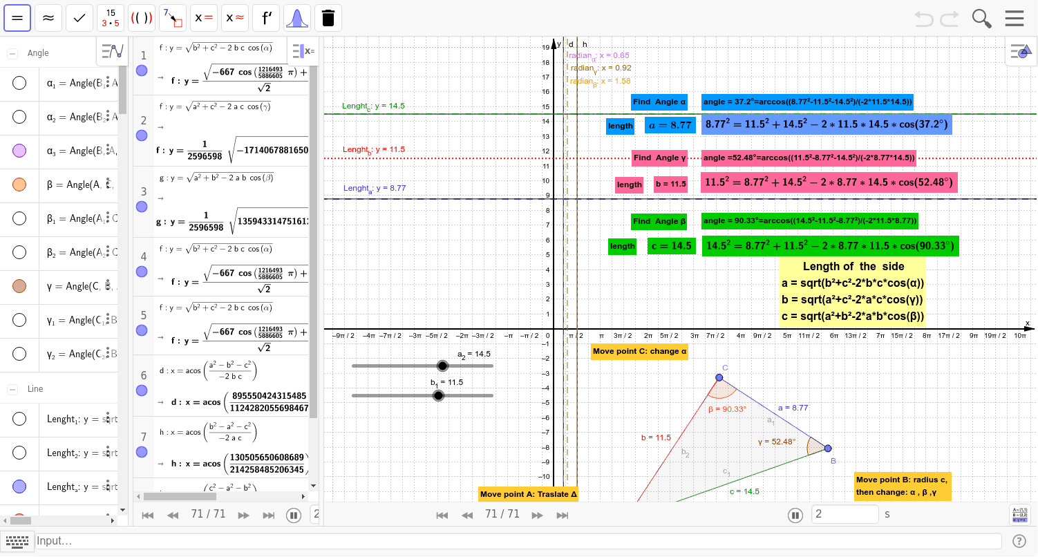
This example dynamically demonstrates the relationship between the sides and an angle of a triangle, visually showcasing the application of the Cosine Theorem. It involves core mathematical concepts such as the Cosine Theorem, triangle geometry, vectors, and functions. The construction uses GeoGebra commands like Point, Segment, Angle, Polygon, and defines objects like a_2, b_1, A, B, c, C, α_3, β, γ, etc., with slider animations to illustrate variations. It is suitable for high school mathematics teaching to help students understand the Cosine Theorem and its application in solving triangles.
GeoGebra Commands & Parameters
Point(Circle[A, a_2]) → BSegment(A, B) → cPoint(Circle[A, b_1]) → CSegment(A, C) → bSegment(C, B) → aAngle(B, A, C) → α_3Angle(A, C, B) → βAngle(C, B, A) → γPolygon(A, C, B) → poly1, b_2, a_1, c_1Point(Circle[A_1, a_2]) → B_1Segment(A_1, B_1) → c_2Point(Circle[A_1, b_1]) → C_1Segment(A_1, C_1) → b_3Segment(C_1, B_1) → a_3Angle(B_1, A_1, C_1) → α_1Angle(A_1, C_1, B_1) → β_1Angle(C_1, B_1, A_1) → γ_1Polygon(A_1, C_1, B_1) → poly1_1, b_4, a_4, c_3Point(Circle[A_2, a_5]) → B_2Segment(A_2, B_2) → c_4Point(Circle[A_2, b_5]) → C_2Segment(A_2, C_2) → b_6Segment(C_2, B_2) → a_6Angle(B_2, A_2, C_2) → α_2Angle(A_2, C_2, B_2) → β_2Angle(C_2, B_2, A_2) → γ_2Polygon(A_2, C_2, B_2) → poly1_2, b_7, a_7, c_5
AI Drawing Prompt Reference
Draw a triangle ABC with vertices A, B, and C, and sides a, b, and c, and angles α, β, and γ. Use circle and point construction methods to create three similar triangles A_1B_1C_1, A_2B_2C_2, and demonstrate changes in angles and side lengths by adjusting sliders.
The prompt above was compiled from the original drawing commands and is for reference only.