
Compound Interest Calculation by Dick Lane
Loading the math board and drawing, please wait…
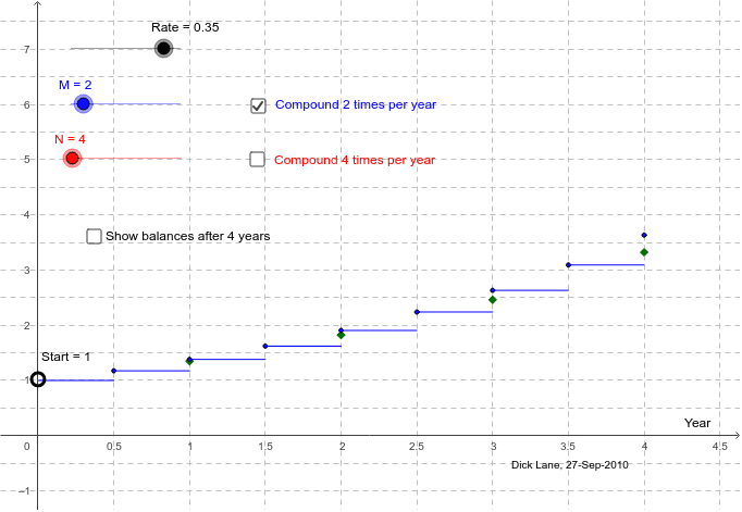
This example demonstrates the step function graph of compound interest, showing how the balance changes over time. Key mathematical concepts include exponential functions and sequences. Using GeoGebra commands such as Point, Sequence, and TableText, you can dynamically explore the effects of different parameters in compound interest calculations. Suitable for high school math education and learning.
GeoGebra Commands & Parameters
Point(yAxis) → SSequence((k, (P * (1 + Rate)^(k))), k, 1, 4) → L1Sequence((k / M, (P * (1 + Rate / M)^(k))), k, 1, (4 * M)) → L2Sequence(Segment[(k / M, (P * RM1^(k))), ((k + 1) / M, (P * RM1^(k)))], k, 0, (4 * M) - 1) → L2aSequence((k / N, (P * (1 + Rate / N)^(k))), k, 1, (4 * N)) → L3TableText(b) → summaryTableSequence(Segment[(k / N, (P * RN1^(k))), ((k + 1) / N, (P * RN1^(k)))], k, 0, (4 * N) - 1) → L3a
AI Drawing Prompt Reference
Draw a step function graph to demonstrate compound interest calculation, including an initial point, three sequences showing account balances at different compounding frequencies over time, and line segments connecting each balance change. Add a table to summarize key data. Start with the initial point, then draw the low-frequency sequence and segments, followed by the high-frequency sequence and segments, and finally add the table.
The prompt above was compiled from the original drawing commands and is for reference only.