
Comparison of Normal and Binomial Distributions
Loading the math board and drawing, please wait…
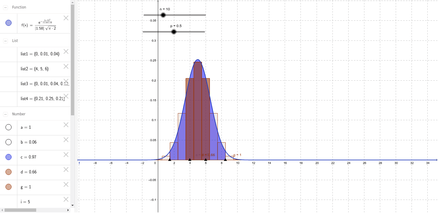
This example visually demonstrates the relationship between normal and binomial distributions. Key mathematical concepts include probability and statistics, specifically normal and binomial distributions. Using GeoGebra commands such as Point, Integral, and BarChart, users can dynamically adjust parameters n and p to observe changes in distribution shapes. Suitable for high school and above students or teachers for teaching and research.
GeoGebra Commands & Parameters
Point(xAxis) → APoint(xAxis) → BIntegral(f, x(A), x(B), true) → cPoint(xAxis) → CPoint(xAxis) → DBarChart({0, 1, 2, 3, 4, 5, 6, 7, 8, 9, 10, 11, 12, 13, 14, 15, 16, 17, 18, 19, 20}, {9.53674316406251E-7, 1.9073486328125E-5, 1.81198120117188E-4, 0.00108718872070313, 0.00462055206298828, 0.0147857666015625, 0.0369644165039064, 0.0739288330078125, 0.120134353637695, 0.160179138183594, 0.176197052001953, 0.160179138183594, 0.120134353637695, 0.0739288330078125, 0.0369644165039064, 0.0147857666015625, 0.00462055206298828, 0.00108718872070313, 1.81198120117188E-4, 1.9073486328125E-5, 9.53674316406251E-7}, 1) → aTake({9.53674316406251E-7, 1.9073486328125E-5, 1.81198120117188E-4, 0.00108718872070313, 0.00462055206298828, 0.0147857666015625, 0.0369644165039064, 0.0739288330078125, 0.120134353637695, 0.160179138183594, 0.176197052001953, 0.160179138183594, 0.120134353637695, 0.0739288330078125, 0.0369644165039064, 0.0147857666015625, 0.00462055206298828, 0.00108718872070313, 1.81198120117188E-4, 1.9073486328125E-5, 9.53674316406251E-7}, x(C) + 1.5, x(D) + 1.5) → list1Take(Sequence[h, h, 0, n], x(C) + 1.5, x(D) + 1.5) → list2BarChart(list2, list1, 1) → bBinomialDist(n, p) → tSequence(BinomialDist[n, p, e, false], e, 0, n) → list3Take(list3, x(C) + 1.5, x(D) + 1.5) → list4BinomialDist(n, p) → gBarChart(list2, list4, 1) → d
AI Drawing Prompt Reference
Create a visualization comparing normal and binomial distributions. Include a smooth normal distribution curve with a shaded area under the curve between point A on the left and point B on the right, representing the probability integral. Below, display a bar chart for the binomial distribution, where each bar's height corresponds to probability values for discrete outcomes. Use points C and D to define the horizontal range of the bar chart. The layout should clearly show the relationship between the distributions, with adjustable parameters n and p for dynamic exploration.
The prompt above was compiled from the original drawing commands and is for reference only.