
Class Scatter Plot and Best Fit Line
Loading the math board and drawing, please wait…
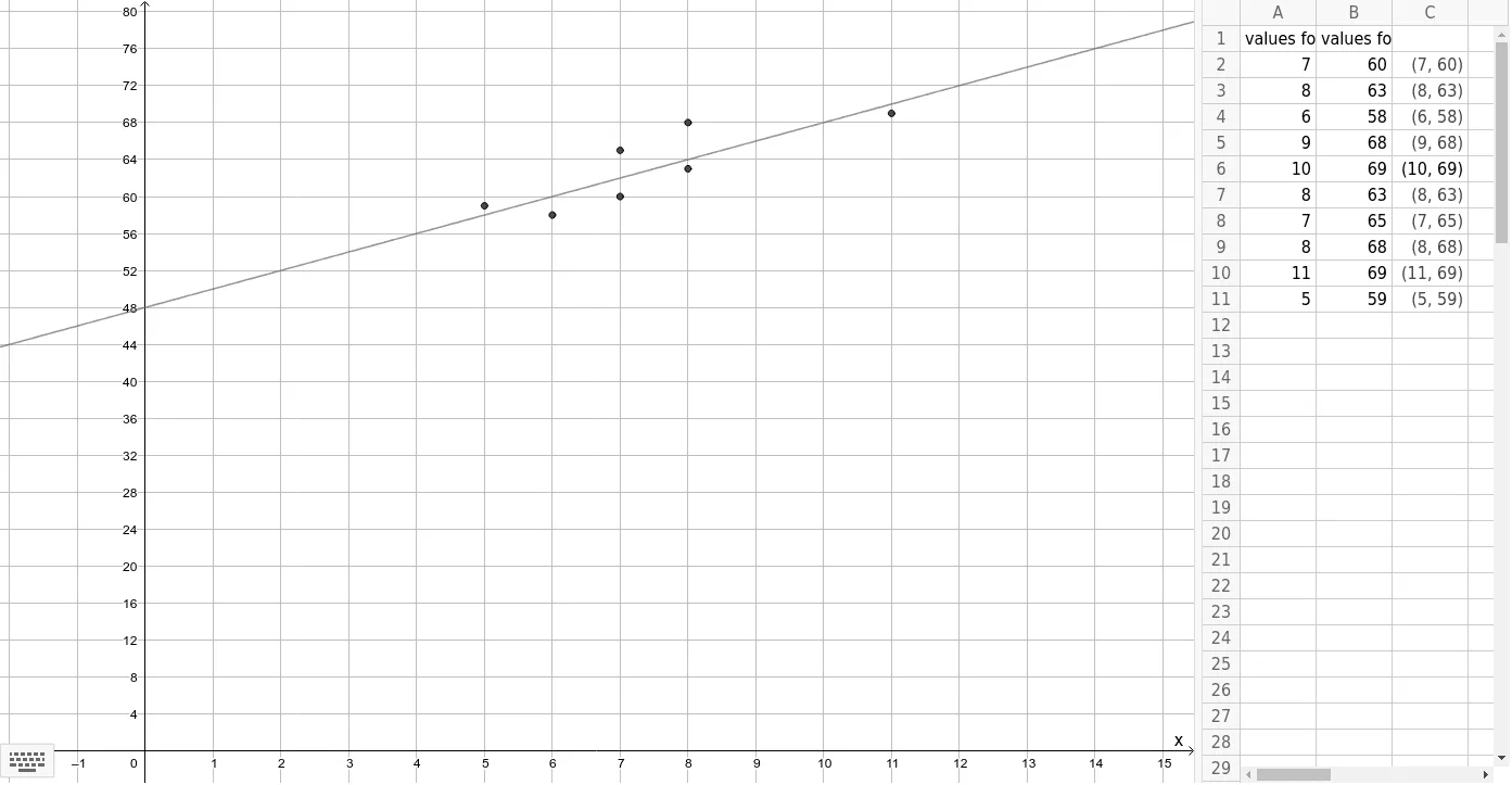
This example demonstrates how to create a scatter plot and draw a best fit line in a classroom setting. Core math concepts include scatter plots, linear regression, best fit lines, and residual analysis. Construction highlights involve GeoGebra commands/objects like ResidualPlot, B7, A7, C7, B2, A2, C2, A4, B4, B3, A3, A1, B1, A5, B5, A6, B6, A8, B8, A9, B9, A10, B10, A11, B11, C4, C3, C5, C8, C6, C9, C10, text1, C11, f. Suitable for high school mathematics and introductory data analysis teaching.
GeoGebra Commands & Parameters
ResidualPlot({(7, 60), (8, 63), (6, 58), (9, 68), (10, 69), (8, 63), (7, 65), (8, 68), (11, 69), (5, 59)}, FitPoly[{(7, 60), (8, 63), (6, 58), (9, 68), (10, 69), (8, 63), (7, 65), (8, 68), (11, 69), (5, 59)}, 1]) →
AI Drawing Prompt Reference
Plot the points (7,60), (8,63), (6,58), (9,68), (10,69), (8,63), (7,65), (8,68), (11,69), (5,59), then draw the best fit line for these points and show the residual plot.
The prompt above was compiled from the original drawing commands and is for reference only.