
Average, Variance, Standard Deviation, and Normal Distribution
Loading the math board and drawing, please wait…
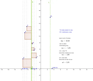
This example demonstrates the calculation of average, variance, and standard deviation, and shows the normal distribution. Key mathematical concepts include average, variance, standard deviation, and normal distribution. Using GeoGebra commands such as OrthogonalLine, Point, Intersect, etc., it provides a clear understanding of these concepts. Suitable for high school mathematics education and learning.
GeoGebra Commands & Parameters
OrthogonalLine(A, xAxis) → aOrthogonalLine(B, xAxis) → bOrthogonalLine(C, xAxis) → cOrthogonalLine(E, xAxis) → dOrthogonalLine(F, xAxis) → eOrthogonalLine(D, xAxis) → fPoint(xAxis) → GOrthogonalLine(G, xAxis) → gOrthogonalLine(A, g) → hIntersect(g, h) → HDistance(A, H) → distanceAHOrthogonalLine(C, g) → mOrthogonalLine(E, g) → nDistance(C, g) → distanceCgIntersect(g, m) → KPolygon(K, C, 4) → poly2, p, q, r, s, L, MIntersect(n, g) → NPolygon(N, E, 4) → poly3, t, a_1, b_1, c_1, O, PPolygon(H, A, 4) → poly1, i, j, k, l, I, JOrthogonalLine(F, g) → d_1Intersect(g, d_1) → QPolygon(Q, F, 4) → poly4, e_1, f_1, g_1, h_1, R, SOrthogonalLine(D, g) → i_1Intersect(g, i_1) → TPolygon(T, D, 4) → poly5, j_1, k_1, l_1, m_1, U, VOrthogonalLine(B, g) → n_1Intersect(g, n_1) → WPolygon(W, B, 4) → poly6, p_1, q_1, r_1, s_1, Z, A_1LaTeX(xav, true, true) → text1LaTeX(ssq, true, true) → text2Intersect(a, xAxis) → D_1Intersect(e, xAxis) → E_1Intersect(f, xAxis) → F_1Intersect(b, xAxis) → G_1Intersect(d, xAxis) → H_1Intersect(c, xAxis) → I_1OrthogonalLine(B_1, xAxis) → t_1LaTeX(var, true, true) → text4LaTeX(sd, true, true) → text5