
Asymmetric Propeller
Loading the math board and drawing, please wait…
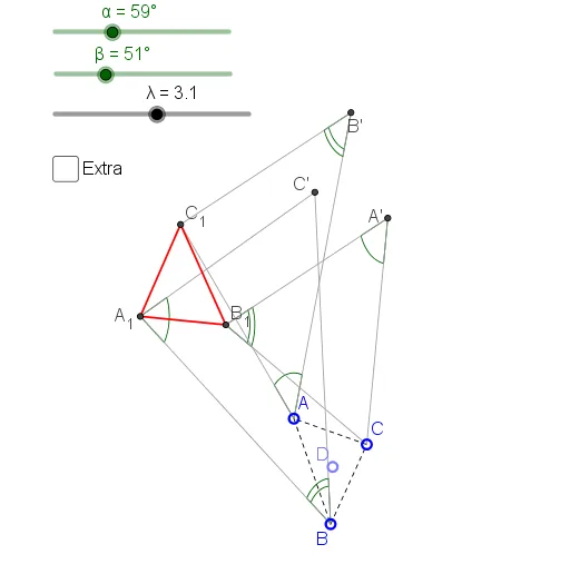
This example demonstrates the geometric construction and dynamic variation of an asymmetric propeller. It involves core mathematical concepts such as Similar Triangles, Triangles, Scatter Plot, Random Experiments, Orthocenter, Normal Distribution, and Integers. The construction utilizes GeoGebra commands and objects like Polygon, Rotate, Ray, Line, Intersect, Segment, Angle, Midpoint, and PointIn. It is suitable for high school mathematics education, showcasing the integration of geometric transformations and data analysis.
GeoGebra Commands & Parameters
Polygon(A, B, C) → poly1, c, a, bRotate(C', β, B) → C''Ray(B, C'') → mLine(C, B') → k_2Rotate(A, (-β), B') → A'_1Ray(B', A'_1) → iRotate(B', α, A) → B''Ray(A, B'') → jIntersect(i, j) → C_1Rotate(B, (-Angle[A, C_1, B']), C') → B'_1Ray(C', B'_1) → nIntersect(m, n) → A_1Line(A_1, C') → n_2Segment(A, B') → fSegment(C', B) → gSegment(C, A') → hSegment(A, C_1) → kSegment(B', C_1) → lSegment(C', A_1) → pSegment(A_1, B) → qRotate(A', Angle[A, C_1, B'], C) → A''Ray(C, A'') → rRotate(C, (-α), A') → C'_1Ray(A', C'_1) → sIntersect(r, s) → B_1Segment(C, B_1) → tSegment(A', B_1) → dSegment(A_1, C_1) → eSegment(B_1, C_1) → f_1Segment(A_1, B_1) → g_1Angle(B, A_1, C') → γAngle(B', A, C_1) → δAngle(B_1, A', C) → εAngle(C_1, B', A) → ζAngle(C, B_1, A') → ηAngle(C', B, A_1) → θAngle(B_1, A_1, C_1) → ιRotate(A, Angle[A, C_1, B'], C') → A'_2Ray(C', A'_2) → h_1Rotate(C', (-α), A) → C''_1Ray(A, C''_1) → i_1Intersect(h_1, i_1) → B_2Segment(C', B_2) → j_1Segment(B_2, A) → k_1Segment(A, C') → l_1Rotate(B', (-Angle[A, C_1, B']), C) → B''_1Ray(C, B''_1) → m_1Rotate(C, β, B') → C'_2Ray(B', C'_2) → n_1Intersect(m_1, n_1) → A_2Segment(B', A_2) → p_1Segment(C, A_2) → q_1Segment(C, B') → r_1Rotate(B, α, A') → B'_2Ray(A', B'_2) → s_1Rotate(A', (-β), B) → A''_1Ray(B, A''_1) → t_1Intersect(s_1, t_1) → C_2Segment(B, C_2) → a_1Segment(C_2, A') → b_1Segment(A', B) → c_1Angle(B_1, A_1, C_1) → κAngle(C_1, B_1, A_1) → μAngle(C', B_2, A) → νAngle(C, B', A_2) → ξAngle(C_2, B, A') → οAngle(B_2, A, C') → ρAngle(B', A_2, C) → σAngle(B, A', C_2) → τSegment(B_2, C_2) → d_1Segment(C_2, A_2) → e_1Segment(A_2, B_2) → f_2Midpoint(A_1, B_1) → E_1Midpoint(B_1, C_1) → F_1Segment(A_1, F_1) → g_2Segment(C_1, E_1) → h_2Intersect(g_2, h_2) → GMidpoint(B_2, A_2) → HMidpoint(A_2, C_2) → ISegment(B_2, I) → i_2Segment(C_2, H) → j_2Intersect(i_2, j_2) → JPointIn(poly1) → KLine(A, C') → l_2Line(C, B_1) → m_2Intersect(l_2, m_2) → EIntersect(k_2, n_2) → FAngle(C', F, C) → υAngle(C', E, C) → ϕAngle(A_1, C', A) → χAngle(B', C, B_1) → ψMidpoint(B, B') → PSegment(B', B) → p_2Segment(C', C) → q_2Segment(A', A) → r_2