Area Bounded by a Polar Curve: Graph and Integral Sum Construction

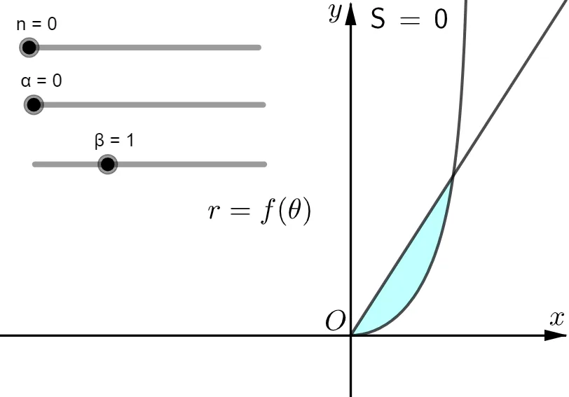
This example demonstrates how to visualize and compute the area enclosed by a polar curve within a specified angular range, using a constructive geometric approach. It highlights the key ideas of polar curves (parameterized by an angle θ), area under/inside a curve, and the link between definite integrals and numerical/segment summation (partition-and-sum approximation). In GeoGebra, the construction is built from rays and the curve (Ray, CurveCartesian), boundary/filled pieces (Polygon), and a generated sequence of sample points or partition elements (Sequence). The area approximation is accumulated using Sum over the discrete slices, while LaTeX labels annotate essential quantities such as angles (α, β, θ), the defining function f, partition markers (c1, c2), reference points (O), slice height terms (h), and parameters like n and Dt for the step size. Suitable for calculus and coordinate-geometry instruction, especially for learning the geometric meaning of integration and area computation via Riemann-sum style visualization.