
Applied Sine & Cosine
Loading the math board and drawing, please wait…
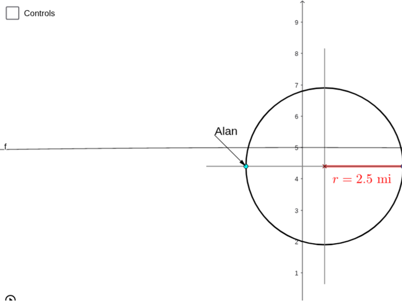
This example demonstrates the application of sine and cosine functions in geometric figures, visually showing the relationship between circles, rays, and points to illustrate the properties of trigonometric functions. Core concepts include trigonometry, vector applications, coordinate geometry transformations, and parametric equations. Constructed using GeoGebra commands like Segment, Circle, Ray, Point, Vector, and objects such as Sequence, Text, and Slider for dynamic interaction. Suitable for high school mathematics teaching to understand the geometric meaning and practical applications of trigonometric functions.
GeoGebra Commands & Parameters
Segment(Alan, P_f) → DistSegCircle(M_1, R) → CCircleArc(M_1, P_i, P_f) → SubArcSegment(M_1, P_i) → rSegSegment(M_1 + (((-R) * 1.5), 0), M_1 + ((R * 1.5), 0)) → xAxSegment(M_1 + (0, ((-1.5) * R)), M_1 + (0, (1.5 * R))) → yAxRay(M_2, M_2 + (1, 0)) → M2rayPoint(M2ray) → M_3Segment(M_2, M_3) → GraphXSegment(M_2 + (0, ((x(M_3) - x(M_2)) * yxVisScale / 2)), M_2 - (0, ((x(M_3) - x(M_2)) * yxVisScale / 8))) → GraphYSequence(Segment[M_2 + (TickL, (((x(M_3) - x(M_2)) * yxVisScale / ((4 * R))) * i)), M_2 + ((-TickL), (((x(M_3) - x(M_2)) * yxVisScale / ((4 * R))) * i))], i, 0, (2 * R)) → yTicksSequence(Text[i, M_2 + ((-0.4), (((x(M_3) - x(M_2)) * yxVisScale / ((4 * R))) * i) - 0.1)], i, 1, (2 * R)) → yLabsSequence(Segment[M_2 + ((((x(M_3) - x(M_2)) * 10) * i / ((120 * π / Rate))), TickL), M_2 + ((((x(M_3) - x(M_2)) * 10) * i / ((120 * π / Rate))), (-TickL))], i, 0, (120 * π / Rate / 10)) → xTicksSequence(Text[(10 * i), M_2 + ((((x(M_3) - x(M_2)) * 10) * i / ((120 * π / Rate))) - 0.2, (-0.4))], i, 1, ((120 * π / Rate)) / 10) → xLabsText("Alan", ATP) → ATVector(ATP, Alan) → AlanVec