Ant on a Cube Activity 2: Paths and Expected Values

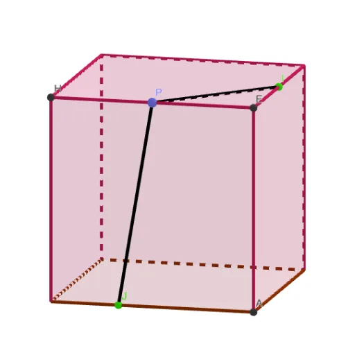
① This example demonstrates an ant moving on the surface of a cube, using a 3D construction to visualize spatial paths and explore stochastic behavior. ② Core mathematical concepts include solid geometry (vertices, edges, faces of a cube), vector operations (representing movement directions and displacements), function graphs (possibly for path length or probability distributions), expected value and stochastic processes (expected number of steps when the ant chooses paths randomly), and hypothesis testing (to test randomness assumptions). ③ Construction highlights: from the summary, GeoGebra commands used include Polygon (to construct faces), Prism (to generate the cube), Vector (to define movement vectors), Midpoint (to find midpoints), and Segment (to connect points); objects include cube vertices A, B, C, D, E, F, G, H, faces face1 to face5, edges edge1 to edge8, vectors vP, vQ, v, and points P, Q, J, etc., with midpoints and vectors building the ant's trajectory. ④ Suitable for high school to early university levels, this serves as interdisciplinary material for solid geometry, vector applications, and probability/statistics (random processes and expected values), ideal for mathematical modeling or inquiry-based learning.