
Acceptance-Rejection Sampling of Normal Distribution
Loading the math board and drawing, please wait…
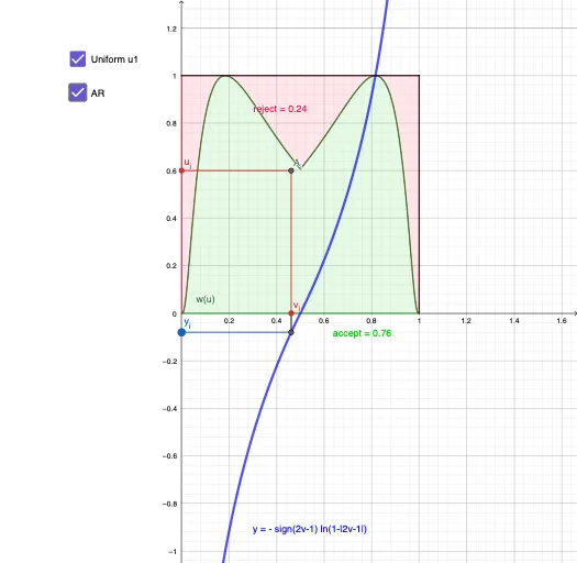
This example demonstrates how to generate normally distributed random numbers using the acceptance-rejection sampling method. Key math concepts include normal distribution, acceptance-rejection sampling algorithm, and integral calculations. GeoGebra commands/objects used in construction are Segment, Point, Intersect, Integral, and IntegralBetween. Suitable for high school and above students to understand sampling methods in probability and statistics.
GeoGebra Commands & Parameters
Segment((0, 1), (1, 1)) → fPoint(xAxis) → v_iIntersect(g, Line[v_i, v_i + (0, 1)], (0.4613402061855664, -0.0804723532225744)) → BPoint(yAxis) → u_iIntersect(Line[u_i, u_i + (1, 0)], Line[v_i, v_i + (0, 1)]) → A_iSegment(v_i, B) → iIntersect(Line[B, B + (1, 0)], yAxis) → y_iSegment(B, y_i) → hSegment(v_i, A_i) → jSegment(A_i, u_i) → kSegment((1, 0), (1, 1)) → lIntegral(w, 0, 1) → acceptIntegralBetween(f, w, 0, 1) → reject
AI Drawing Prompt Reference
Draw the acceptance-rejection sampling for a normal distribution. Start by drawing a horizontal line segment, then take a point on the x-axis and find point B by intersecting the line through this point and a unit vector with the horizontal line. Next, take a point on the y-axis and find point A_i by intersecting the line through this point and point B with the y-axis. Connect points v_i and B, B and y_i, v_i and A_i, A_i and u_i, and (1,0) and (1,1). Calculate the integral from 0 to 1 of line segment f and the integral difference from w to 1 of f, representing the accept and reject areas.
The prompt above was compiled from the original drawing commands and is for reference only.