
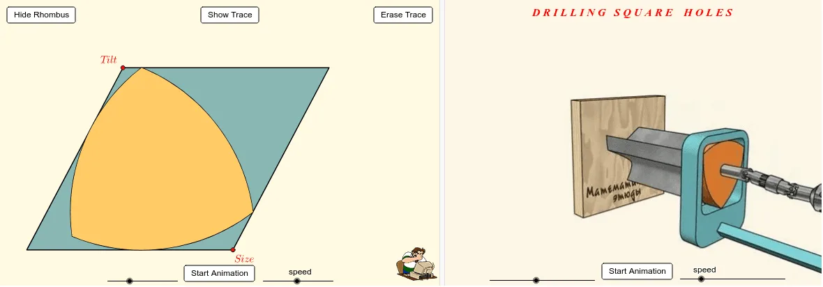
A Rolling Reuleaux Triangle in a Rhombus
Loading the math board and drawing, please wait…
This example visualizes the rolling motion of a Reuleaux triangle inside a rhombus, demonstrating constant-width curve geometry, relative motion, and locus generation. Core mathematical concepts include Reuleaux polygon properties, circular arcs, angle rotation, and differential geometry of rolling curves. Construction utilizes GeoGebra commands such as Ray, Point, Rotate, Mirror, Circle, Intersect, Translate, and objects like angle, distance, vector, circle arc, and polygon tools. Suitable for high school advanced geometry, calculus transition units, or parametric curve exploration.
GeoGebra Commands & Parameters
Ray(A, A') → aa'Point(aa') → BRotate(B, (-betta), B) → B'Mirror(B, A) → BBCircle(BB, A) → bbaCircle(A, B) → abIntersect(ab, bba, 2) → DRotate(D, (-betta), B) → D'Rotate(B, delta, D) → KCircle(K, K2) → kk2Translate(D', Vector[B, K]) → D''Translate(B', Vector[B, K]) → B''Ray(B'', D'') → bd''Intersect(kk2, bd'') → K1,Angle(K1, K, K2) → kIntersect(ab, bba, 1) → CDistance(C, D) → cdVector(K, M) → kmTranslate(D, km) → D1Rotate(D1, k, M) → D2Translate(C, km) → C1Rotate(C1, k, M) → C2Translate(B, km) → B1Rotate(B1, k, M) → B2Translate(A, km) → A1Rotate(A1, k, M) → A2Ray(M, M') → mm'Point(mm') → NRotate(N, π / 10, M) → N'Rotate(N, π / 2, M) → Q'CircleArc(M, N', Q') → nq'Point(nq') → QOrthogonalLine(N, Line[M, Q]) → nIntersect(Line[M, Q], n) → LDistance(N, L) → nlDilate(D2, c, M) → D3Dilate(C2, c, M) → C3Translate(C3, Vector[N, L]) → C4Dilate(B2, c, M) → B3Line(D3, B3) → d3b3Line(C4, d3b3) → c4Dilate(A2, c, M) → A3Line(A3, C3) → a3c3Ray(B, D) → bdRay(B', D') → bd'Translate(N, Vector[M, Q]) → PPolyLine(M, N, P, Q, M) → mLine(B3, A3) → b3a3Circle(C3, B3) → c3b3Line(C3, D3) → c3d3Translate(B3, Vector[N, L]) → B4Line(B4, b3a3) → b4Intersect(c3d3, b4) → RAffineRatio(D3, C3, R) → dcrDilate(B4, dcr1, D3) → B5AffineRatio(C3, D3, R) → cdrDilate(B5, cdr1, C3) → B6Translate(B6, Vector[N, L]) → B7Line(B6, B7) → b6b7Intersect(a3c3, d3b3) → TRay(C3, A3) → c3a3Intersect(c3b3, c3a3) → U,Intersect(a3c3, c4) → SAffineRatio(T, U, S) → tusDilate(C4, tus1, U) → C5OrthogonalLine(C5, d3b3) → c5Intersect(d3b3, c5) → VAffineRatio(D3, B3, V) → dbvDilate(C5, dbv1, D3) → C6OrthogonalLine(C6, b6b7) → c6Intersect(b6b7, c6) → EAffineRatio(B6, B7, E) → beDilate(C6, be1, B6) → C7Intersect(Line[M, Q], b6b7) → FTranslate(A3, Vector[C7, F]) → A4Line(A4, Line[M, Q]) → a4Line(A3, Line[M, N]) → a3Intersect(a3, a4) → GTranslate(C3, Vector[A3, G]) → V2Translate(B3, Vector[A3, G]) → V1Translate(D3, Vector[A3, G]) → V3CircleArc(V1, V3, V2) → v132CircleArc(V2, V1, V3) → v213CircleArc(V3, V2, V1) → v321Distance(M, N) → dLine(I, xAxis) → iPoint(i) → JPolygon({M, N, P, Q}) → m1CircleSector(V1, V3, V2) → v1CircleSector(V2, V1, V3) → v2CircleSector(V3, V2, V1) → v3