3D Parametric Surface Tiling with Function Fitting

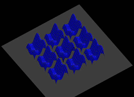
① This example demonstrates a 3D tiling-like structure generated by parametric surfaces and sequences, combined with polynomial fitting to connect discrete points into continuous curves, merging solid geometry with function graphing. ② Core mathematical concepts include parametric equations, surface construction, sequence generation, polynomial fitting, and translation transformations, touching on indefinite integrals (via fitted curves) and scatter plot correlation. ③ Construction highlights: from the summary, commands such as Point (defining points A-I), FitPoly (creating polynomial f), CurveCartesian (parametric curves), Surface (3D surfaces), and Sequence (e.g., liste2) are used, with sliders n and m controlling tiling density and extent, achieving a 3D tiled effect through translation and scaling. ④ Suitable for high school to university levels, useful for teaching solid geometry, parametric equations, function fitting, and computational geometric design, as well as an engaging case for exploring 3D pattern generation and mathematical modeling.