
球体与锥体交互演示
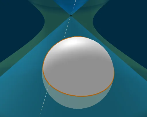
几何画板及绘图内容加载中,请稍等……
①本范例演示球体与锥体的交互形成的几何图形与轨迹;②涉及核心数学概念包括解析几何、立体几何、参数方程、导数与极限;③作图要点运用了 Sphere(球体)、IntersectPath(路径交点)、Intersect(交点)、Point(点)、Line(直线)、Locus(轨迹)、Coefficients(系数)、OrthogonalPlane(正交平面)、OrthogonalLine(正交直线)等 GeoGebra 命令与对象;④适合高中及以上学生及数学爱好者用于理解空间几何与高等数学概念。
GeoGebra 命令及参数
Sphere((K_x, 0, -3 + K_h), (K_x, 0, K_h)) → KIntersectPath(a, QuK) → dIntersect(zAxis, yAxis) → InfPoint(d) → ALine(Inf, A) → fIntersect(f, K, 2) → BLocus(B, A) → Ortslinie1Intersect(e, d) → C_x, D_xIntersect(b, d) → E_y, F_yCoefficients(d) → Koeff_dIntersect(f, K) → C, DLocus(C, A) → Ortslinie2Coefficients(QuK) → ListQuIntersectPath(e, j) → lIntersectPath(e, k) → mSphere(((-λ_M), 0, (-0.81 * λ_M)), (0, 0, 0)) → K_pOrthogonalPlane(Q_p, l) → nIntersectPath(n, QuK) → pIntersect(f, n) → HPoint(p) → P_PLine(Inf, P_P) → qIntersect(q, K_p, 2) → ILocus(I, P_P) → Ortslinie3Intersect(f, K, 1) → EIntersectPath(e, zyl) → gOrthogonalLine(KPKT, e) → sIntersect(s, zyl) → G,Intersect(g, K) → J, N, ,Intersect(s, K) → L, MOrthogonalPlane(L, s) → oIntersectPath(o, K) → rOrthogonalLine(M, s, space) → f_1OrthogonalLine(M, s, space) → g_1OrthogonalLine(M, s, space) → h_1OrthogonalLine(M, s, space) → i_1OrthogonalLine(M, s, space) → j_1OrthogonalLine(M, s, space) → k_1OrthogonalPlane(M, s) → tIntersectPath(t, zyl) → c_1
AI 绘图提示语参考
画一个球体与圆锥体相交的图形,展示它们形成的几何形状和轨迹。球体位于圆锥内部,两者相交产生曲线。先画出球体和圆锥,然后求出它们的交线,再利用交线画出轨迹。最后,通过轨迹和交点构造出两条曲线,并添加辅助线和平面,展示空间几何关系和高级数学概念。
以上提示语为根据原始绘图命令整理而来,仅供参考。