
勾股定理探索 by mcalpiho
几何画板及绘图内容加载中,请稍等……
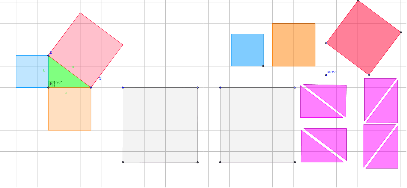
①本范例演示直角三角形三边平方和关系;②核心数学概念为勾股定理;③作图要点:使用Line, OrthogonalLine, Intersect, Polygon, Angle, Point, Segment, Rotate等GeoGebra命令构建图形;④适合初中及以上学生用于理解勾股定理及几何作图。
GeoGebra 命令及参数
Line(S, D) → LOrthogonalLine(R, L) → MOrthogonalLine(E, L) → NIntersect(L, N) → FPolygon(E, F, D) → poly1, b, a, cAngle(D, F, E) → αPolygon(D, F, 4) → poly2, f, g, h, i, F_1, GPolygon(F, E, 4) → poly3, j, k, l, m_2, H, IPolygon(E, D, 4) → poly4, n_2, p, q, r, J, KPoint(Circle[V, a + b]) → WSegment(V, W) → mPoint(Circle[Z, a + b]) → A_1Segment(Z, A_1) → nPolygon(A_1, Z, 4) → poly8, i_1, j_1, k_1, l_1, B_1, C_1Polygon(W, V, 4) → poly9, m_1, n_1, p_1, q_1, D_1, E_1Point(Circle[K_2, a]) → L_2Point(Circle[M_2, a]) → N_2Line(K_2, L_2) → a_4Point(Circle[K_2, b]) → P_2Line(M_2, N_2) → d_4Point(Circle[M_2, b]) → R_2Point(Circle[S_2, a]) → T_2Point(Circle[S_2, b]) → U_2Point(Circle[V_2, a]) → W_2Segment(V_2, W_2) → i_4Point(Circle[V_2, b]) → Z_2Segment(V_2, Z_2) → j_4Polygon(Z_2, V_2, W_2) → poly20, w_2, z_2, v_2Point(Circle[G_3, a]) → H_3Segment(G_3, H_3) → h_4Point(Circle[G_3, b]) → I_3Segment(G_3, I_3) → m_4Polygon(I_3, G_3, H_3) → poly21, h_5, i_5, g_5Angle(poly20) → θ, ι, κAngle(poly21) → ϕ, χ, ψPoint(Circle[A_3, a]) → B_3Segment(A_3, B_3) → s_3Rotate(B_3, 90*°, A_3) → C_3Angle(B_3, A_3, C_3) → δSegment(C_3, A_3) → t_3Point(Circle[A_3, b]) → D_3Segment(A_3, D_3) → b_4Polygon(D_3, A_3, B_3) → poly17, b_5, d_5, a_5Point(Circle[E_3, a]) → F_3Segment(E_3, F_3) → c_4Point(Circle[E_3, b]) → J_3Segment(E_3, J_3) → e_4Angle(J_3, E_3, F_3) → εPolygon(J_3, E_3, F_3) → poly18, f_4, j_5, e_5Point(Circle[K_3, a]) → L_3Segment(K_3, L_3) → g_4Point(Circle[K_3, b]) → M_3Segment(K_3, M_3) → k_4Angle(L_3, K_3, M_3) → ζPolygon(M_3, K_3, L_3) → poly19, l_4, m_5, k_5Point(Circle[N_3, a]) → O_3Segment(N_3, O_3) → n_4Point(Circle[N_3, b]) → P_3Segment(N_3, P_3) → p_4Angle(O_3, N_3, P_3) → ηPolygon(O_3, N_3, P_3) → poly22, p_5, o_3, n_5Point(Circle[A, a]) → BSegment(A, B) → dPoint(Circle[A, b]) → CSegment(A, C) → ePoint(Circle[O, a]) → PSegment(O, P) → sPoint(Circle[O, b]) → QSegment(O, Q) → tAngle(B, A, C) → βPolygon(B, C, A) → poly5, a_1, b_1, c_1Angle(P, O, Q) → γPolygon(P, O, Q) → poly6, q_2, p_2, oPoint(Circle[T, a]) → USegment(T, U) → d_1Point(Circle[G_1, b]) → H_1Segment(G_1, H_1) → e_1Polygon(U, T, 4) → poly7, g_1, h_1, r_1, s_1, K_1, L_1Polygon(H_1, G_1, 4) → poly10, t_1, a_2, b_2, c_2, M_1, N_1Point(Circle[MOVE, a]) → R_1Segment(MOVE, R_1) → h_2Rotate(R_1, 90*°, MOVE) → S_1Angle(R_1, MOVE, S_1) → λOrthogonalLine(S_1, h_2) → i_2Point(Circle[MOVE, b]) → T_1Segment(MOVE, T_1) → j_2Angle(R_1, MOVE, T_1) → μOrthogonalLine(T_1, h_2) → k_2Polygon(T_1, MOVE, R_1) → poly12, r_2, t_2, q_3Line(MOVE, R_1) → l_2Line(T_1, l_2) → d_3Polygon(T_1, R_1, 4) → poly13, s_2, a_3, b_3, c_3, V_1, W_1
AI 绘图提示语参考
画一个直角三角形,并在每条边上分别绘制一个正方形。通过比较三个正方形的面积来展示勾股定理。首先画出直角三角形,然后画出每条边上的正方形,并标注出每个正方形的面积。接着,画出从直角顶点到斜边中点的线段,并展示其长度关系。最后,通过旋转和镜像等操作,进一步验证勾股定理的几何意义。
以上提示语为根据原始绘图命令整理而来,仅供参考。