
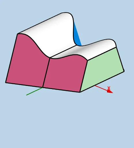
可修改立体:平行于y轴的等腰梯形截面
几何画板及绘图内容加载中,请稍等……
本范例演示一个由上下两条函数曲线围成的立体,其所有平行于y轴的截面均为等腰梯形,且梯形的较长底边等于上函数值减去下函数值。核心数学概念是积分学中的截面法求体积,通过动态调整上下函数、旋转角度和高度等参数,直观展示立体形状随截面变化的过程。作图要点包括:使用Line、Ray、Circle、Segment等构造基础几何元素,通过Rotate、Translate、Mirror实现空间变换,利用CurveCartesian和Surface生成曲面,并借助Textfield、Slider等交互控件实现参数调节。该范例适合高中至大学阶段学习微积分、立体几何和函数图像的学生,帮助理解截面面积与体积积分的关系。
GeoGebra 命令及参数
Line(I, I + (1, 0, 0)) → f_1Rotate(H, (ANG * pi / 180), I, f_1) → H'Rotate(I, ((-ANG) * pi / 180), H, Plane[H', I, H]) → I'_1Ray(H, I'_1) → p_2Ray(I, H') → q_2Intersect(q_2, p_2) → W_1Circle(W_1, (SLratio * Distance[W_1, I]), Plane[W_1, I, H]) → e_2Intersect(q_2, e_2) → B_2, C_2Intersect(p_2, e_2) → Z_1, A_2Line(K, K + (1, 0, 0)) → tRotate(J, (ANG * pi / 180), K, t) → J'_1Ray(K, J'_1) → k_2Rotate(K, ((-ANG) * pi / 180), J, Plane[J'_1, K, J]) → K'Ray(J, K') → j_2Intersect(k_2, j_2) → R_1Circle(R_1, (SLratio * Distance[R_1, K]), Plane[J'_1, K, J]) → d_2Intersect(j_2, d_2) → U_1, V_1Intersect(k_2, d_2) → S_1, T_1Intersect(lower, h, (0, -9)) → CLine(C, C + (1, 0, 0)) → cIntersect(upper, h, (0, 5)) → BSegment(C, B) → qIntersect(upper, q, (0, 5)) → GRotate(G, (ANG * pi / 180), C, c) → G'_1Rotate(C, (ANG * pi / 180), G, Plane[G, C, G'_1]) → C'Ray(G, C') → f_2Ray(C, G'_1) → g_2Intersect(g_2, f_2) → M_1Circle(M_1, (SLratio * Distance[M_1, C]), Plane[C, G'_1, G]) → c_2Intersect(g_2, c_2) → N_1, O_1Intersect(f_2, c_2) → P_1, Q_1Translate(G'_1, Vector[C, G]) → J_1Segment(H, I) → s_1Midpoint(s_1) → A_1Segment(J, K) → q_1Midpoint(q_1) → ZMidpoint(s_1) → EMidpoint(q_1) → FMidpoint(C, G) → TLine(B, D) → iSphere(B, d) → eSegment(C, B) → pTextfield(upper) → InputBox1Textfield(lower) → InputBox2Textfield(a) → InputBox3Textfield(b) → InputBox4Segment(C, G) → k_1Line(C, G) → jSphere(G, T) → kLine(T, T + (1, 0, 0)) → mRotate(G, pi / 3, F_1, m) → G'Rotate(G', pi / 3, F_1, Line[F_1, F_1 + (1, 0, 0)]) → G''Line(F_1, F_1 + (1, 0, 0)) → nPolygon(C, G, Q_1, O_1) → poly1, g_1, m_1, r_1, a_1Rotate(G'', pi / 3, F_1, n) → G'''Rotate(G''', pi / 3, F_1, n) → G_1Line(Z, Z + (1, 0, 0)) → fLine(D_1, D_1 + (1, 0, 0)) → gRotate(J, pi / 3, D_1, g) → J'Rotate(J', pi / 3, D_1, g) → J''Rotate(J'', pi / 3, D_1, g) → J'''Rotate(J''', pi / 3, D_1, g) → E_1Line(H_1, H_1 - (1, 0, 0)) → l_1Rotate(I, pi / 3, H_1, l_1) → I'Rotate(I', pi / 3, H_1, l_1) → I''Rotate(I'', pi / 3, H_1, l_1) → I'''Rotate(I''', pi / 3, H_1, l_1) → I_1Translate(J'_1, Vector[K, J]) → K_1Polygon(K, J, V_1, T_1) → q1, j_1, l_2, m_2, n_2Polygon(I, H, A_2, C_2) → q2, e_1, h_2, i_2, f_3Translate(H', Vector[I, H]) → H''Intersect(t, q_1) → L_1Angle(G, C, G'_1) → αSegment(O_1, Q_1) → rSegment(G, Q_1) → lAngle(Q_1, G, C) → βSegment(O_1, C) → sSegment(T_1, L_1) → d_1Segment(J, V_1) → b_1Segment(T_1, V_1) → c_1Segment(C_2, I) → p_1Segment(H, A_2) → i_1Segment(A_2, C_2) → n_1CurveCartesian(t, (0.5 * (upper(t) + lower(t))) - ((SLratio * 0.5) * (upper(t) - lower(t))), ((((1 - SLratio) * 0.5) * (upper(t) - lower(t))) * tan((ANG * pi / 180))), t, a, b) → oCurveCartesian(t, (0.5 * (upper(t) + lower(t))) + ((SLratio * 0.5) * (upper(t) - lower(t))), ((((1 - SLratio) * 0.5) * (upper(t) - lower(t))) * tan((ANG * pi / 180))), t, a, b) → uSurface(u, lower(u) + ((((1 - SLratio) * 0.5) * (upper(u) - lower(u))) * v), (((((1 - SLratio) * 0.5) * (upper(u) - lower(u))) * tan((ANG * pi / 180))) * v), u, a, b, v, 0, 1) → o_1Surface(u, upper(u) - ((((1 - SLratio) * 0.5) * (upper(u) - lower(u))) * v), (((((1 - SLratio) * 0.5) * (upper(u) - lower(u))) * tan((ANG * pi / 180))) * v), u, a, b, v, 0, 1) → u_1Surface(u, lower(u) + (((1 - SLratio) * 0.5) * (upper(u) - lower(u))) + ((SLratio * (upper(u) - lower(u))) * v), ((((1 - SLratio) * 0.5) * (upper(u) - lower(u))) * tan((ANG * pi / 180))), u, a, b, v, 0, 1) → v_1Mirror(o_1, Plane[(0, 0, 0), (1, 0, 0), (1, 1, 0)]) → w_1Mirror(o, Plane[(0, 0, 0), (1, 0, 0), (1, 1, 0)]) → o'Mirror(u_1, Plane[(0, 0, 0), (1, 0, 0), (1, 1, 0)]) → a_2Mirror(v_1, Plane[(0, 0, 0), (1, 0, 0), (1, 1, 0)]) → b_2Mirror(J, Plane[(0, 0, 0), (1, 0, 0), (1, 1, 0)]) → J'_2Mirror(V_1, Plane[(0, 0, 0), (1, 0, 0), (1, 1, 0)]) → D_2Segment(J'_2, D_2) → r_2Mirror(T_1, Plane[(0, 0, 0), (1, 0, 0), (1, 1, 0)]) → E_2Mirror(L_1, Plane[(0, 0, 0), (1, 0, 0), (1, 1, 0)]) → F_2Segment(E_2, F_2) → s_2Mirror(T_1, Plane[(0, 0, 0), (1, 0, 0), (1, 1, 0)]) → G_2Mirror(V_1, Plane[(0, 0, 0), (1, 0, 0), (1, 1, 0)]) → H_2Segment(G_2, H_2) → t_2Mirror(poly1, Plane[(0, 0, 0), (1, 0, 0), (1, 1, 0)]) → poly1'Mirror(O_1, Plane[(0, 0, 0), (1, 0, 0), (1, 1, 0)]) → I_2Mirror(C, Plane[(0, 0, 0), (1, 0, 0), (1, 1, 0)]) → C'_1Segment(I_2, C'_1) → s'Mirror(O_1, Plane[(0, 0, 0), (1, 0, 0), (1, 1, 0)]) → J_2Mirror(Q_1, Plane[(0, 0, 0), (1, 0, 0), (1, 1, 0)]) → K_2Segment(J_2, K_2) → r'Mirror(G, Plane[(0, 0, 0), (1, 0, 0), (1, 1, 0)]) → G'_2Mirror(Q_1, Plane[(0, 0, 0), (1, 0, 0), (1, 1, 0)]) → L_2Segment(G'_2, L_2) → l'Mirror(u, Plane[(0, 0, 0), (1, 0, 0), (1, 1, 0)]) → u'Mirror(q1, Plane[(0, 0, 0), (1, 0, 0), (1, 1, 0)]) → q1'Mirror(q2, Plane[(0, 0, 0), (1, 0, 0), (1, 1, 0)]) → q2'Mirror(C_2, Plane[(0, 0, 0), (1, 0, 0), (1, 1, 0)]) → M_2Mirror(I, Plane[(0, 0, 0), (1, 0, 0), (1, 1, 0)]) → I'_2Segment(M_2, I'_2) → g_3Mirror(H, Plane[(0, 0, 0), (1, 0, 0), (1, 1, 0)]) → H'_1Mirror(A_2, Plane[(0, 0, 0), (1, 0, 0), (1, 1, 0)]) → N_2Segment(H'_1, N_2) → h_3Mirror(A_2, Plane[(0, 0, 0), (1, 0, 0), (1, 1, 0)]) → O_2Mirror(C_2, Plane[(0, 0, 0), (1, 0, 0), (1, 1, 0)]) → P_2Segment(O_2, P_2) → i_3Angle(J_2, C, G) → γAngle(L_2, G, C) → δTextfield(SLratio) → InputBox5
AI 绘图提示语参考
绘制一个三维立体图形,其垂直于y轴的截面为等腰梯形。该立体由上下两条函数曲线界定,梯形的较长底边等于上下函数之差。通过滑块调整上下函数、旋转角度和高度,观察截面变化。图形包含两个主要截面区域,每个区域由两条射线和圆弧构成,形成对称的梯形轮廓。立体表面由多个平面和曲面拼接而成,并显示关键点、线段和角度标记。整体呈现动态可调的几何体,用于演示积分求体积的截面法。
以上提示语为根据原始绘图命令整理而来,仅供参考。