二项分布动态演示：概率直方图与正态近似

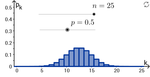
This GeoGebra example dynamically illustrates the binomial distribution's probability mass function and its approximation by the normal distribution. ① It demonstrates how the probability histogram of a binomial distribution approaches a bell-shaped normal curve as the number of trials n increases, visually conveying the central limit theorem. ② Core mathematical concepts include the binomial distribution, probability mass function, expected value μ=np, standard deviation σ=√(npq), continuity correction, and normal approximation. ③ Construction highlights: the Join and Sequence commands generate discrete point sequences; objects d, p, q, n, f, Plotf, mu, sigma, and n_max are defined, where p is the success probability, n is the number of trials, f is the probability function, Plotf renders the histogram, mu and sigma compute distribution parameters, and n_max controls the maximum trials for dynamic adjustment. ④ Suitable for high school to early college probability and statistics courses, it helps students explore how the binomial distribution's shape changes with parameters, the conditions for normal approximation, and interactive statistical concepts via sliders.