Water Volume (RO) – Binomial Distribution and Riemann Sums in a Random Experimen

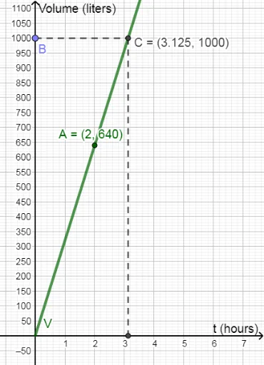
This GeoGebra example dynamically simulates a random experiment for water volume, visually linking the binomial distribution with upper and lower Riemann sums. It demonstrates how random sampling and geometric constructions can illustrate the convergence of discrete probability to continuous integration. Core concepts include volume, binomial distribution, circumcircle, dilation (homothety), random experiments, and Riemann sums (upper and lower). The construction uses commands such as Point to define key points V, A, B, OrthogonalLine to create perpendicular lines g, Intersect to find points C and D, and Segment to draw segments i and j, forming an interactive model. Suitable for high school to undergraduate students, this example helps learners grasp the approximation of binomial probabilities, numerical integration via Riemann sums, and the interplay between geometric transformations and stochastic processes.