
Unit Tangent, Normal, and Binormal Vectors (Frenet Frame) Dynamic Demo
Loading the math board and drawing, please wait…
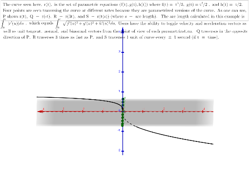
This GeoGebra example dynamically visualizes the unit tangent vector T, unit normal vector N, and unit binormal vector B (the Frenet frame) along a parametric space curve. It demonstrates the local geometry of curves in 3D, highlighting concepts such as tangent direction, curvature, torsion, and the orthonormal basis attached to each point. The construction uses the CurveCartesian command to define the parametric curve, Vector commands to draw the three vectors, and Integral commands for arc-length-related computations. Numerous derivative objects (f', g', h', etc.) and vector operations (T, N, B) are built, with a slider s controlling the moving point on the curve to update the frame in real time. This is ideal for university-level calculus or differential geometry courses, as well as advanced high school enrichment, to intuitively grasp the Frenet-Serret formulas and the meaning of curvature and torsion.
GeoGebra Commands & Parameters
CurveCartesian((f(t), g(t), h(t)), t, -10, 10) → r_{0}Vector(P, P + (f'(t), g'(t), h'(t))) → r'Vector(P, P + UnitVector[r']) → TVector(P, P + (F'(t), G'(t), H'(t))) → T'Vector(P, P + UnitVector[T']) → NVector(P, P + T ⊗ N) → BCurveCartesian(f((-t)), g((-t)), h((-t)), t, -10, 10) → r_{1}CurveCartesian(f((3 * t)), g((3 * t)), h((3 * t)), t, -10, 10) → r_{2}Integral(sqrt(f'(t)^(2) + g'(t)^(2) + h'(t)^(2)), 0, t) → sVector(Q, Q + (f_{1}'(t), g_{1}'(t), h_{1}'(t))) → v_{1}Vector(Q, Q + (f_{1}''(t), g_{1}''(t), h_{1}''(t))) → a_{1}Vector(R, R + (f_{2}'(t), g_{2}'(t), h_{2}'(t))) → v_{2}Vector(S, S + (f_{3}'(s), g_{3}'(s), h_{3}'(s))) → v_{3}Vector(S, S + (f_{3}''(s), g_{3}''(s), h_{3}''(s))) → a_{2}Vector(S, S + (f_{3}''(s), g_{3}''(s), h_{3}''(s))) → a_{3}Vector(Q, Q + UnitVector[v_{1}]) → T_{1}Vector(R, R + UnitVector[v_{2}]) → T_{2}Vector(S, S + UnitVector[v_{3}]) → T_{3}Vector(Q, Q + (F'((-t)), G'((-t)), H'((-t)))) → T_{1}'Vector(R, R + (F'((3 * t)), G'((3 * t)), H'((3 * t)))) → T_{2}'Vector(S, S + (F'(s), G'(s), H'(s))) → T_{3}'Vector(Q, Q + UnitVector[T_{1}']) → N_{1}Vector(R, R + UnitVector[T_{2}']) → N_{2}Vector(S, S + UnitVector[T_{3}']) → N_{3}Vector(Q, Q + T_{1} ⊗ N_{1}) → B_{1}Vector(R, R + T_{2} ⊗ N_{2}) → B_{2}Vector(S, S + T_{3} ⊗ N_{3}) → B_{3}CurveCartesian(r_{0}(((cbrt(2) * (sqrt((36 * s^(2)) + 2) + (6 * s))^(2 / 3)) - 2^(2 / 3)) / ((2 * cbrt(sqrt((36 * s^(2)) + 2) + (6 * s))))), s, -10, 10) → r_{3}
AI Drawing Prompt Reference
Draw a 3D space curve with its Frenet frame, including the unit tangent vector T, unit normal vector N, and unit binormal vector B. Define the curve using parametric equations, compute and draw T, N, and B, and demonstrate the local geometry of the curve, such as tangent direction, curvature, and torsion. Use a slider to control the point on the curve and dynamically update the frame.
The prompt above was compiled from the original drawing commands and is for reference only.