
Tangent Field and Solution Curve Exploration
Loading the math board and drawing, please wait…
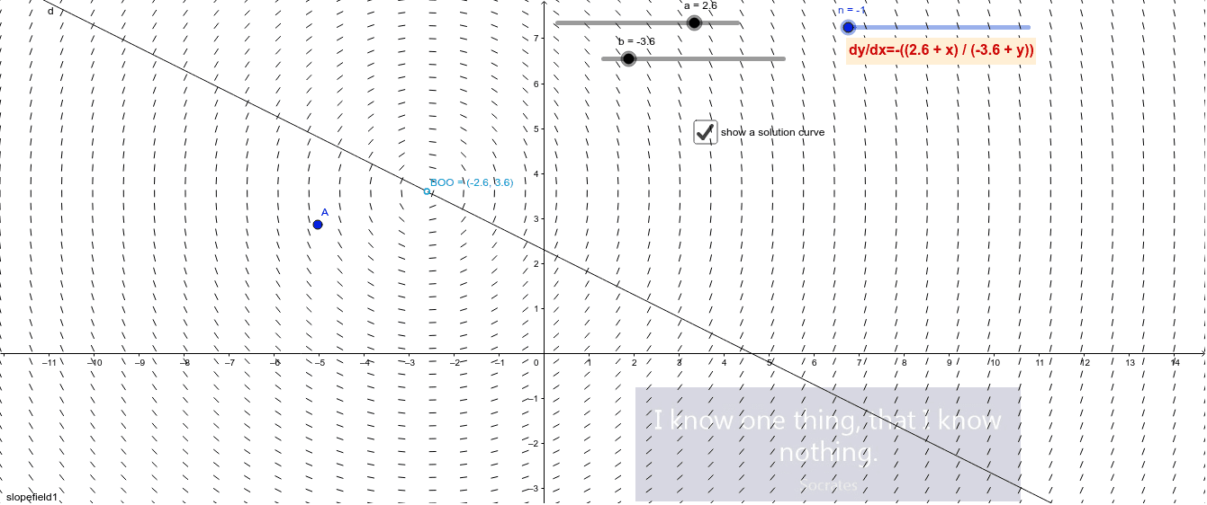
This example demonstrates how to visualize solution curves of differential equations through tangent fields. Core math concepts include differential equations, vector fields, and solution curves. Key GeoGebra commands used are SlopeField and SolveODE to plot the tangent field and solve the differential equations, with parameters n, b, a adjustable via sliders. Suitable for high school and above students to learn and understand the geometric meaning of differential equations, ideal for teaching demonstrations and exploratory learning.
GeoGebra Commands & Parameters
SlopeField(f) → slopefield1SolveODE(f, A) → g
AI Drawing Prompt Reference
Draw a coordinate plane with a slope field generated by a differential equation, using short line segments to indicate tangent directions at each point. Place a starting point on the plane and draw a solution curve that follows the slope field from that point, representing the integral curve of the equation. Include adjustable parameters to control the density of the field and the extent of the curve, allowing dynamic exploration of how the solution changes with different initial conditions.
The prompt above was compiled from the original drawing commands and is for reference only.