
Spreadsheet, Graphing, and Statistics Integration Example
Loading the math board and drawing, please wait…
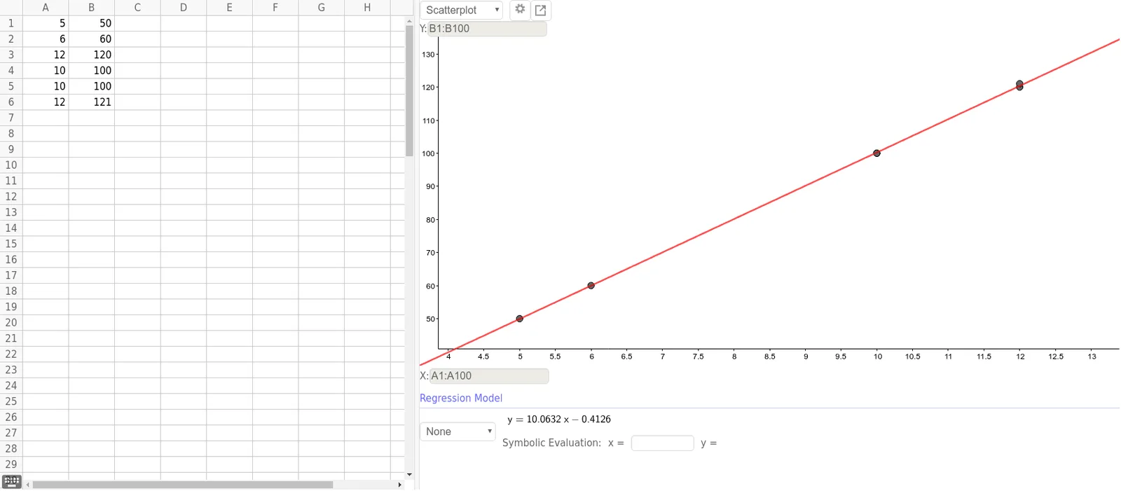
①This example demonstrates how to integrate spreadsheet data, function graphing, and statistical analysis tools in a single GeoGebra workspace, using a residual plot to visually show the fit of data to a model. ②Core mathematical concepts include linear functions, median value, inequalities, special points (such as residual points), and statistical measures, involving basic ideas of data visualization and regression analysis. ③Construction highlights: From the construction summary, the ResidualPlot command is used, referencing multiple spreadsheet cell objects (A1 to B6) that store data points; the residual plot is generated based on these data, possibly combined with linear function graphs and inequality regions for auxiliary analysis. ④Suitable for middle school or introductory statistics courses, helping students understand data distribution, linear fitting, and residuals, and also useful for teachers demonstrating the linkage between spreadsheets and graphs in teaching scenarios.
GeoGebra Commands & Parameters
ResidualPlot({(5, 50), (6, 60), (12, 120), (10, 100), (10, 100), (12, 121)}, FitPoly[{(5, 50), (6, 60), (12, 120), (10, 100), (10, 100), (12, 121)}, 1]) →
AI Drawing Prompt Reference
Create a scatter plot with data points and a fitted linear function, including a residual plot based on the same data. Use distinct colors for data points and the fitted curve, and highlight residual points. Add inequality regions for auxiliary analysis to visually demonstrate data distribution, linear fitting, and residuals, suitable for statistical teaching to show the connection between data and graphs.
The prompt above was compiled from the original drawing commands and is for reference only.