
Solving a system of equations with possible multiple solutions
Loading the math board and drawing, please wait…
In collections
Linear Algebra
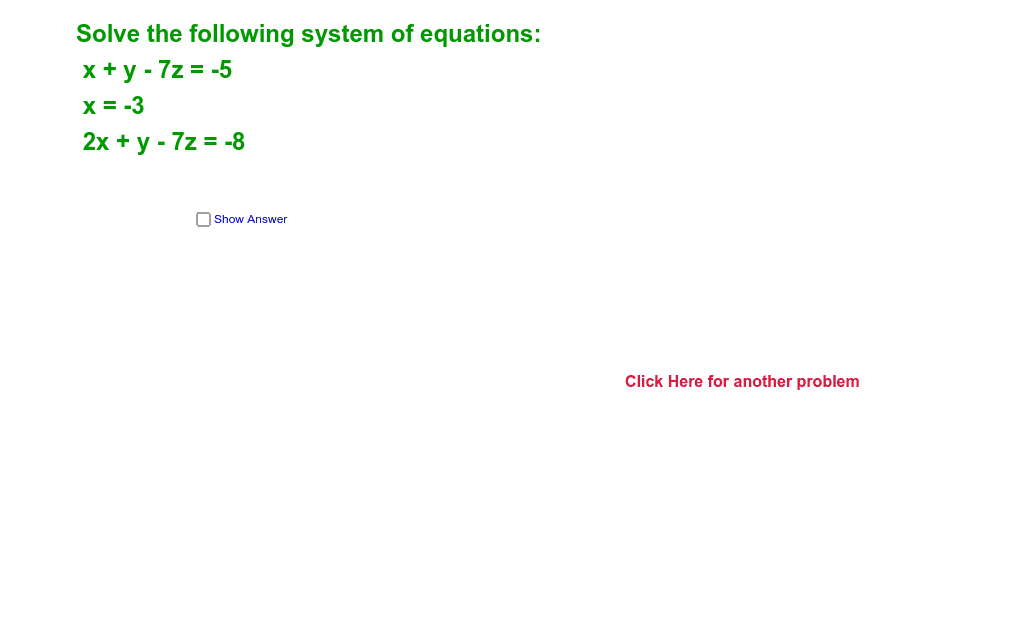
This example demonstrates how to construct and analyze systems of equations in GeoGebra, highlighting the concept of multiple solutions. Key mathematical concepts include the existence and uniqueness of solutions, parameter influence, and geometric interpretation. Construction involves using RandomElement, Random, If, and LaTeX commands to generate random parameters and display solution variations. Suitable for high school students or college undergraduates to understand the geometric meaning of equation solutions and their applications in coordinate geometry and calculus.
GeoGebra Commands & Parameters
RandomElement({0, 1}) → c34Random(-7, 7) → c12Random(-7, 7) → c13Random(-7, 7) → c23Random(-7, 7) → c14Random(-7, 7) → c24Random(-7, 7) → cRandom(-3, 3) → qRandom(-3, 3) → sRandom(-4, 4) → rElement({"Reduced Row Echelon Form Of", "transpose of", "scalar multiple of"}, pick) → opElement({ReducedRowEchelonForm[A3], Transpose[A3], (c * A3)}, pick) → CElement(C, 1, 4) → x1Element(C, 2, 4) → y1Element(C, 3, 4) → z1If(Element[C1, 3, 3] ≟ Element[C1, 3, 4], "Infinite Number of Solutions", "No solution") → text3Element(C1, 2, 4) → y21Element(C1, 2, 3) → y22Element(C1, 1, 4) → x21Element(C1, 1, 3) → x22LaTeX(C1) → text7
AI Drawing Prompt Reference
Draw a graph of a system of equations with random parameters. The graph should include random parameter points, representations of solution sets, and descriptions of possible solutions. The construction order should start with generating parameters, then showing the equation system, and finally presenting the geometric meaning of solutions.
The prompt above was compiled from the original drawing commands and is for reference only.