
Sine Transformations: Exploring Dynamic Changes in Trigonometric Graphs
Loading the math board and drawing, please wait…
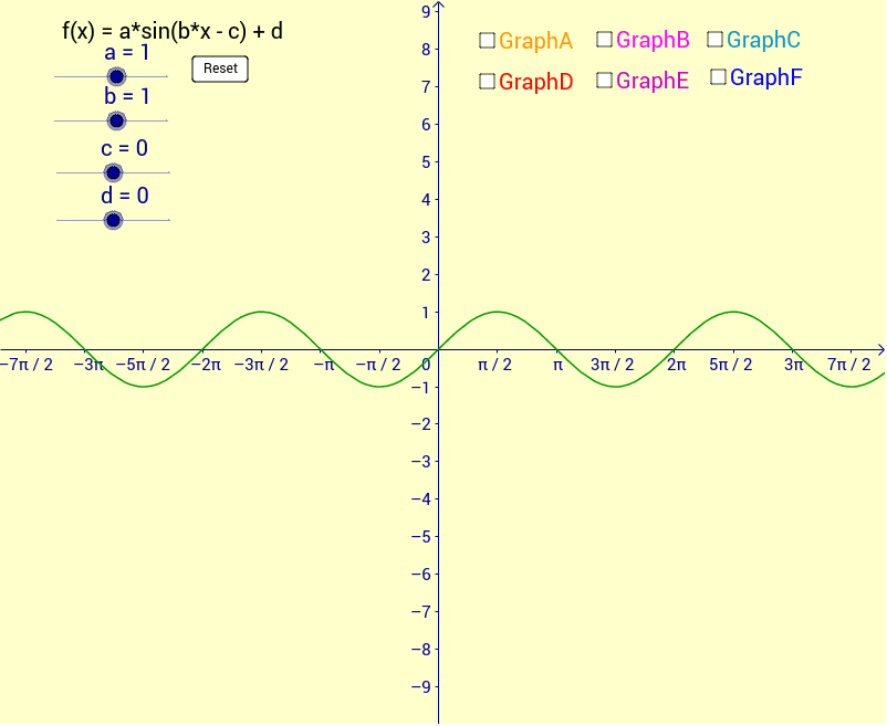
This example demonstrates the dynamic changes in trigonometric graphs through sine transformations. Key mathematical concepts include trigonometric function properties, image transformation rules, and coordinate system applications. Construction involves using GeoGebra commands like GraphA, h, i, j to build function graphs, combined with text annotations to explain transformation processes. Suitable for high school math classes or middle school geometry teaching to understand dynamic changes in trigonometric functions.
GeoGebra Commands & Parameters
Numeric a(1.0)Numeric b(1.0)Numeric c(0.0)Numeric d(0.0)f(x) = a * sin(b * (x - c)) + dg(x) = 2 * sin(x) - 3Boolean GraphA(false)h(x) = 3 * sin(x + 1.57) + 1Boolean i(false)j(x) = -2 * sin(x - 1.57) + 3Boolean e(false)k(x) = sin(4 * x) - 2Boolean l(false)m(x) = 5 * sin(2 * x - 0.785) - 4Boolean n(false)p(x) = -0.75 * sin(0.5 * x) + 1Boolean o(false)