
Relationship between Average and Standard Deviation
Loading the math board and drawing, please wait…
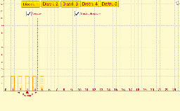
This example illustrates the relationship between average and standard deviation. It involves key statistical concepts such as mean and standard deviation. Using GeoGebra commands like Vector, Polygon, Mean, etc., it provides a visual representation of data distribution characteristics. Suitable for high school mathematics education, particularly in statistics and probability courses.
GeoGebra Commands & Parameters
Vector((0, 1)) → uVector((0.5, 0)) → vPolygon(C, C + v, C + v + u, C + u, C) → polígono1, b, c, d, e, fPolygon(D, D + v, D + v + u, D + u, D) → polígono2, d_1, g, h, i, d_2Polygon(A, A + v, A + v + u, A + u, A) → polígono3, a_1, j, k, l, a_2Polygon(E, E + v, E + v + u, E + u, E) → polígono4, e_1, m, n, p, e_2Polygon(F, F + v, F + v + u, F + u, F) → polígono5, f_1, q, r, s, f_2Polygon(G, G + v, G + v + u, G + u, G) → polígono6, g_1, t, b_1, c_1, g_2Polygon(H, H + v, H + v + u, H + u, H) → polígono7, h_1, i_1, j_1, k_1, h_2Polygon(I, I + v, I + v + u, I + u, I) → polígono8, i_2, l_1, m_1, n_1, i_3Polygon(J, J + v, J + v + u, J + u, J) → polígono9, j_2, p_1, q_1, r_1, j_3Polygon(K, K + v, K + v + u, K + u, K) → polígono10, k_2, a, s_1, t_1, k_3Mean({x(A), x(C), x(D), x(E), x(F), x(G), x(H), x(I), x(J), x(K)}) → oRay(L, M) → b_2Point(xAxis) → NRay(L, N) → c_2Sequence(Text[i, (0.18, 0) + (Vector[(1, 0)] * i)], i, 0, 50) → lista3Vector(B, B + (o_1, 0)) → v_1Segment(B + (o_1, 0.25), B + (o_1, 10.25)) → l_2Segment(B + ((-o_1), 0.25), B + ((-o_1), 10.25)) → m_2Vector(B, B + ((-o_1), 0)) → w_1