Polar Curve r=a+b·cos(θ) with Dynamic Parameters

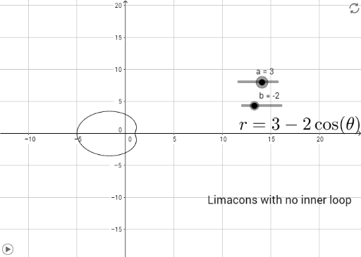
① This example demonstrates how to plot the polar curve r=a+b·cos(θ) for θ from 0 to 2π, which can produce classic shapes such as limaçons and cardioids. ② The core mathematical concepts include polar coordinates, conversion to Cartesian coordinates, parametric equations, trigonometric periodicity, and the influence of parameters a and b on the curve's shape. ③ Construction details: The GeoGebra command CurveCartesian is used to convert the polar equation into a parametric curve, with an If condition to restrict the θ range; sliders control a and b for dynamic exploration, text objects display current parameter values, and auxiliary points A1, A2, B1, B2 are constructed to mark key positions. ④ Suitable for high school to early college students, this example helps understand polar geometry, parametric curve plotting, and dynamic mathematical exploration, and can serve as a classroom demonstration or self-study tool.