
Minimization of Least Squares via Different Regularization Procedures
Loading the math board and drawing, please wait…
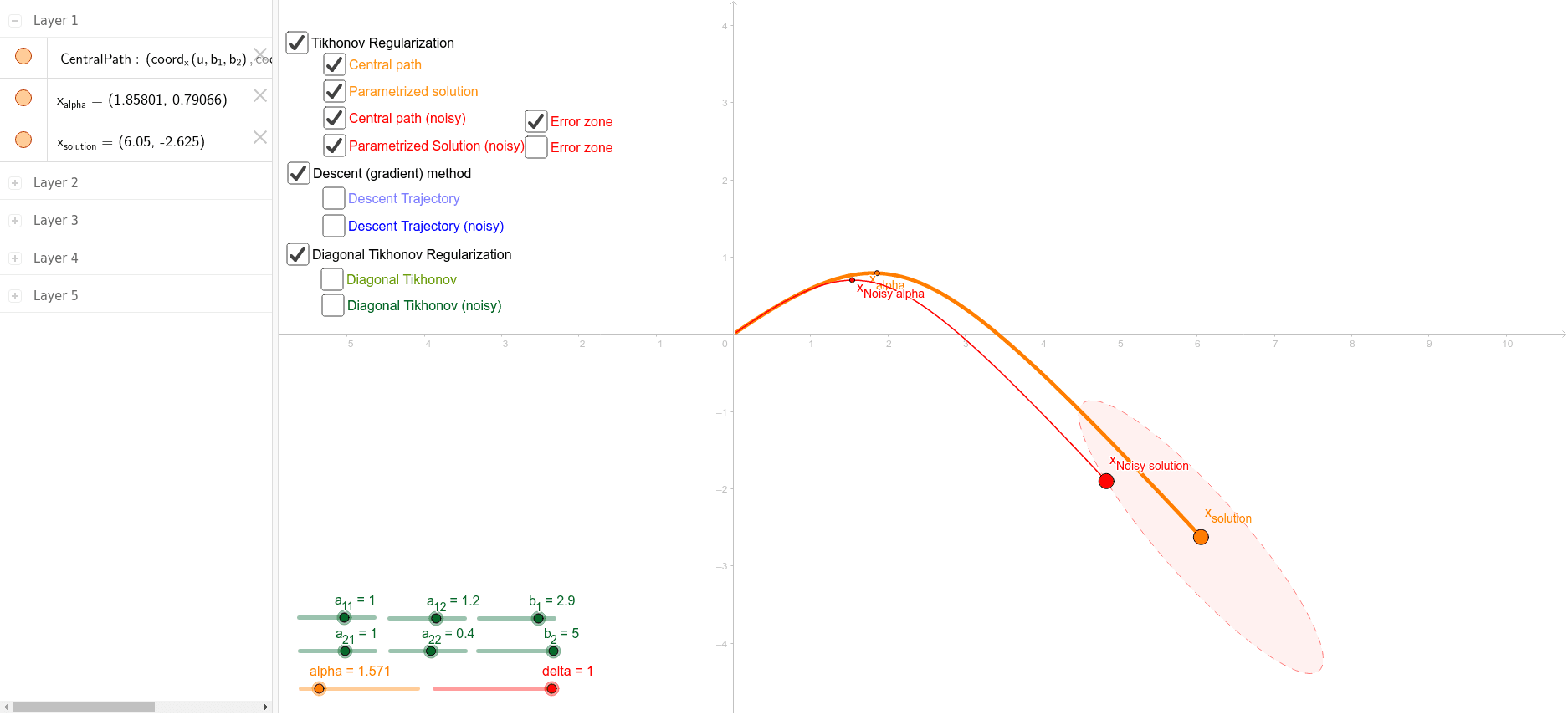
This GeoGebra example demonstrates the minimization of the least squares functional f(x)=0.5*||Ax-b||^2 for a 2x2 matrix A and 2x1 vector b, focusing on how different regularization procedures affect the solution path. It visualizes the central path, noisy solution areas, and stopping rules in the presence of random noise. Core mathematical concepts include least squares, regularization (e.g., Tikhonov), singular value decomposition (SVD), noise perturbation, and solution stability. The construction uses GeoGebra commands such as RandomNormal to generate noise, CurveCartesian to plot the central path and noisy regions, and If to implement stopping rules. Key objects include matrix A, vector b, noise vectors, SVD components (U, V, eigenvalues lambda), and regularization parameter alpha. This is suitable for university-level linear algebra, numerical analysis, or optimization courses, helping students visualize the trade-off between fitting error and solution norm, and the impact of noise on regularized solutions.
GeoGebra Commands & Parameters
RandomNormal(0, delta) → rand_yRandomNormal(0, delta) → rand_xCurveCartesian((coord_x(u, b_1 + x(epsilon), b_2 + y(epsilon)), coord_y(u, b_1 + x(epsilon), b_2 + y(epsilon))), u, 0, 200) → NoisyCentralPathCurveCartesian((coord_x(u, b_1, b_2), coord_y(u, b_1, b_2)), u, 0, 200) → CentralPathIf(lambda_1 ≠ 0, 1 / lambda_1, 0) → invLambda_1If(lambda_2 ≠ 0, 1 / lambda_2, 0) → invLambda_2CurveCartesian(x(x_{solution}) + exptAA_x(t, x(x_0) - x(x_{solution}), y(x_0) - y(x_{solution})), y(x_{solution}) + exptAA_y(t, x(x_0) - x(x_{solution}), y(x_0) - y(x_{solution})), t, 0, NumberIterationSteepestDescent) → SteepestDescentCurveCartesian(x(x_{Noisy solution}) + exptAA_x(t, x(x_0) - x(x_{Noisy solution}), y(x_0) - y(x_{Noisy solution})), y(x_{Noisy solution}) + exptAA_y(t, x(x_0) - x(x_{Noisy solution}), y(x_0) - y(x_{Noisy solution})), t, 0, NumberIterationSteepestDescent) → NoisySteepestDescentCurveCartesian((1 / (1 + t) * exptAA_x(t, x(x_0 - x_{solution}) + invtAA_x(x(x_{solution}), y(x_{solution})), y(x_0 - x_{solution}) + invtAA_y(x(x_{solution}), y(x_{solution})))) - (1 / (1 + t) * invtAA_x(x(x_{solution}), y(x_{solution}))) + x(x_{solution}), (1 / (1 + t) * exptAA_y(t, x(x_0 - x_{solution}) + invtAA_x(x(x_{solution}), y(x_{solution})), y(x_0 - x_{solution}) + invtAA_y(x(x_{solution}), y(x_{solution})))) - (1 / (1 + t) * invtAA_y(x(x_{solution}), y(x_{solution}))) + y(x_{solution}), t, 0, (2 * NumberIterationSteepestDescent)) → DiagonalTikhonov_1CurveCartesian((1 / (1 + t) * exptAA_x(t, x(x_0 - x_{Noisy solution}) + invtAA_x(x(x_{Noisy solution}), y(x_{Noisy solution})), y(x_0 - x_{Noisy solution}) + invtAA_y(x(x_{Noisy solution}), y(x_{Noisy solution})))) - (1 / (1 + t) * invtAA_x(x(x_{Noisy solution}), y(x_{Noisy solution}))) + x(x_{Noisy solution}), (1 / (1 + t) * exptAA_y(t, x(x_0 - x_{Noisy solution}) + invtAA_x(x(x_{Noisy solution}), y(x_{Noisy solution})), y(x_0 - x_{Noisy solution}) + invtAA_y(x(x_{Noisy solution}), y(x_{Noisy solution})))) - (1 / (1 + t) * invtAA_y(x(x_{Noisy solution}), y(x_{Noisy solution}))) + y(x_{Noisy solution}), t, 0, (2 * NumberIterationSteepestDescent)) → NoisyDiagonalTikhonov
AI Drawing Prompt Reference
Create a mathematical illustration showing the minimization of the least squares functional f(x)=0.5*||Ax-b||^2, highlighting the central path and noisy solution areas affected by random noise. The visualization should emphasize how different regularization procedures impact the solution path, including noise perturbations and stopping rules. Key elements are a 2x2 matrix, a 2x1 vector, noise vectors, SVD components (U, V, eigenvalues), and a regularization parameter. Plot the central path and noisy regions as curves, and depict regularization paths via iterative descent methods to show solution stability.
The prompt above was compiled from the original drawing commands and is for reference only.