
Interactive Linear Regression by GeoGebra Institute of Southern Connecticut
Loading the math board and drawing, please wait…
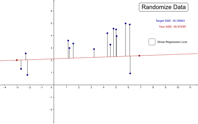
This example demonstrates how to interactively find a line that minimizes the sum of squared errors through linear regression. Key math concepts include linear regression, least squares method, and residual analysis. GeoGebra commands and objects used in construction are Line, Mean, Sum, OrthogonalLine, Intersect, Segment, and Residual. Suitable for high school and above students to understand the process of building a linear regression model.
GeoGebra Commands & Parameters
Line(A, B) → aMean(A2:A16) → A18Mean(B2:B16) → B18Sum(F2:F16) → F18Sum(G2:G16) → G18Line(D, C) → bOrthogonalLine(O11, xAxis) → cIntersect(b, c) → ESegment(E, O11) → dResidual(O1, b) → eResidual(O2, b) → fResidual(O10, b) → gResidual(O3, b) → hResidual(O12, b) → iResidual(O4, b) → jResidual(O13, b) → kResidual(O5, b) → lResidual(O14, b) → mResidual(O6, b) → nResidual(O8, b) → pResidual(O15, b) → qResidual(O9, b) → rResidual(O7, b) → sResidual(O10, a) → tResidual(O11, a) → a_1Residual(O1, a) → b_1Residual(O2, a) → c_1Residual(O12, a) → d_1Residual(O3, a) → e_1Residual(O13, a) → f_1Residual(O4, a) → g_1Residual(O14, a) → h_1Residual(O5, a) → i_1Residual(O6, a) → j_1Residual(O15, a) → k_1Residual(O7, a) → m_1Residual(O8, a) → n_1Residual(O9, a) → p_1Sum(I2:I16) → I18Sum(J2:J16) → J18
AI Drawing Prompt Reference
Draw a scatter plot to demonstrate linear regression by minimizing the sum of squared errors. First, plot the best-fit line, then show all residuals from data points to this line. Also, calculate and display residuals of all data points to the best-fit line and the mean line. Finally, draw a perpendicular line from the mean point to the best-fit line and mark its intersection point.
The prompt above was compiled from the original drawing commands and is for reference only.